第 8 章 神经网络
8.1 神经网络的基本概念
8.1.1 神经元
神经元是神经网络的基本单元。一个神经元由输入端、组合函数、激活函数、输出端组成。组合函数和激活函数是神经网络的核心。
knitr::include_graphics("https://vnote-1251564393.cos.ap-chengdu.myqcloud.com/typora-img/20220420092837.png")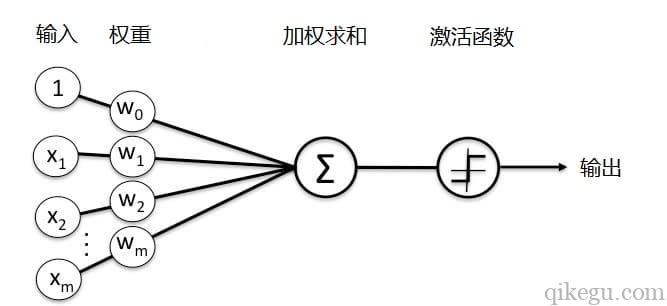
图 8.1: 神经元的结构
人工神经元是一个基于生物神经元的数学模型,神经元接受多个输入信息,对它们进行加权求和,再经过一个激活函数处理,然后将这个结果输出。
对于神经网络而言,神经元节点本身相当于一个神经细胞,输入相当于树突,带权重的连接相当于轴突,输出相当于突触5。
8.1.2 多层感知器
多个神经元连接在一起就形成了神经网络。多层感知器是一种常用的神经网络。各个自变量通过输入层的神经元输入到网络,输入层的输出传递给隐藏层,作为后者的输入;数据经过多个隐藏层的传递后,最终被转换后的数据在输出层形成输出值。
多层感知器通常在隐藏层使用线性组合函数和 S 型激活函数,在输出层使用线性组合函数和与因变量相适应的激活函数。
多层感知器可以形成很复杂的非线性模型。只要给予足够的数据、隐藏层和训练时间,含一层隐藏层的多层感知器就能够以任意精确度近似自变量和因变量之间几乎任何形式的函数;使用多个隐藏层可能用更少的隐藏神经元和参数就能形成复杂的非线性模型,提高模型的泛化能力6。
除了多层感知器,常见的神经网络还包括:卷积神经网络、循环神经网络等。卷积神经网络(CNN)旨在解决图像识别问题,卷积神经网络在图像识别、推荐系统以及自然语言处理等方面有着广泛的应用。循环神经网络在语音识别、生成图像描述、音乐合成和机器翻译等领域有着广泛的应用。
不同类型的神经网络都是由多个神经元连接而成的,其主要区别在于神经元的连接规则不同。
对于多层感知器而言,其连接规则为:
- 神经元按照层来布局。最左边的输入层,负责接收输入数据;最右边的输出层,负责输出数据。
- 中间是隐藏层,对于外部不可见。隐藏层可以包含多层,大于一层的就被称为深度神经网络,层次越多数据处理能力越强。
- 同一层的神经元之间没有连接。
- 前后两层的所有神经元相连,前层神经元的输出就是后层神经元的输入。
- 每个连接都有一个权值。
knitr::include_graphics("https://vnote-1251564393.cos.ap-chengdu.myqcloud.com/typora-img/20220420100007.png")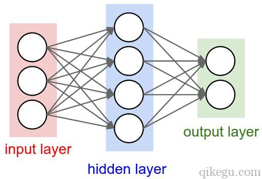
8.1.3 组合函数和激活函数
组合函数通常用线性组合函数,其实就是一个简单的按权重加和。
\[u_j = \sum(v_1, ..., v_s) = b_j + \sum_{r=1}^sw_{rj}v_r\]
激活函数是非线性函数,对组合函数的结果进行处理。它的可选类型比较多,主要有:
-
S 型函数
- Logistic 函数:\(y = \frac{1}{1+e^{-x}} \in (0, 1)\)
- Tanh 函数(双曲正切函数):\(y = 1 - \frac{2}{1+e^{2x}} \in (-1, 1)\)
- Eliot 函数(Softsign 函数):\(y = \frac{x}{1+|x|} \in (-1, 1)\)
- Arctan 函数:\(y = \frac{2}{\pi}arctan(x) \in (-1,1)\)
ReLU 函数(线性整流函数):(8.1)
\[\begin{equation} f(x) = \begin{cases} x & \text{if } x \geq 0 \\ 0 & \text{if } x < 0 \end{cases} \tag{8.1} \end{equation}\]
- Softmax 函数:\(y_j = \frac{e^{u_j}}{\sum_{j'=1}^je^{u_{j'}}} \in (0,1)\)
与 S 型函数和 ReLu 函数不同,Softmax 函数是多变量输入激活函数。Softmax 与正常的 max 函数不同:max 函数仅输出最大值,但 Softmax 确保较小的值具有较小的概率,并且不会直接丢弃。
这些激活函数都能将组合函数产生的 \((-\infty, \infty)\) 通过单调连续的非线性转换变成有限的输出值。每种函数在运算速度、可微性、输出值等方面存在差异,因此具有不同的应用场景。
8.1.4 神经网络的训练
神经网络的训练,就是求解组合函数权重的过程。简单来说就是从基于误差函数,对权重值不断进行修正,最终是误差逐渐趋近为 0 的过程。误差函数越小,模型拟合效果越好。
根据因变量的取值类型,要在输出层选用不同的激活函数。
- 因变量是二值变量或比例,输出层激活函数采用 Logistic 函数;
- 因变量是多种取值的定类变量,输出层激活函数使用 Softmax 函数或 Logistic 函数;
- 因变量是多种取值的定序变量,可将其看做定类变量,或者根据多个输出单元的结果进行定序;
- 因变量为计数变量(事件发生的次数),输出层的激活函数采用指数函数;
- 因变量为取值可正可负的连续变量(如满足正态分布的数值),输出层激活函数采用恒等函数;
- 因变量为非负连续变量(如收入、销售额),通常将因变量进行 Box-Cox 转换后,在使用因变量可正可负的方法。
这部分内容解释起来比较复杂,暂且略过
8.2 使用神经网络预测红酒品质
ch7_wine.csv 记录了与红酒品质相关的 12 个变量,分别是:
- fixed.acidity:固定酸度
- volatile.acidity:挥发性酸度
- citric.acid:柠檬酸
- residual.sugar:残留的糖分
- chlorides:氯化物
- free.sulfur.dioxide:游离二氧化硫
- total.sulfur.dioxide:总二氧化硫
- density:密度
- pH:酸碱度
- sulphates:硫酸盐
- alcohol:酒精度
- quality:因变量,品质等级,取值 3 - 9。
file = xfun::magic_path("ch7_wine.csv")
wine = readr::read_csv(file)
wine
## # A tibble: 4,898 × 12
## fixed…¹ volat…² citri…³ resid…⁴ chlor…⁵ free.…⁶ total…⁷ density pH sulph…⁸
## <dbl> <dbl> <dbl> <dbl> <dbl> <dbl> <dbl> <dbl> <dbl> <dbl>
## 1 7 0.27 0.36 20.7 0.045 45 170 1.00 3 0.45
## 2 6.3 0.3 0.34 1.6 0.049 14 132 0.994 3.3 0.49
## 3 8.1 0.28 0.4 6.9 0.05 30 97 0.995 3.26 0.44
## 4 7.2 0.23 0.32 8.5 0.058 47 186 0.996 3.19 0.4
## 5 7.2 0.23 0.32 8.5 0.058 47 186 0.996 3.19 0.4
## 6 8.1 0.28 0.4 6.9 0.05 30 97 0.995 3.26 0.44
## 7 6.2 0.32 0.16 7 0.045 30 136 0.995 3.18 0.47
## 8 7 0.27 0.36 20.7 0.045 45 170 1.00 3 0.45
## 9 6.3 0.3 0.34 1.6 0.049 14 132 0.994 3.3 0.49
## 10 8.1 0.22 0.43 1.5 0.044 28 129 0.994 3.22 0.45
## # … with 4,888 more rows, 2 more variables: alcohol <dbl>, quality <dbl>, and
## # abbreviated variable names ¹fixed.acidity, ²volatile.acidity, ³citric.acid,
## # ⁴residual.sugar, ⁵chlorides, ⁶free.sulfur.dioxide, ⁷total.sulfur.dioxide,
## # ⁸sulphates
## # ℹ Use `print(n = ...)` to see more rows, and `colnames()` to see all variable names8.2.1 数据标准化和拆分
将数据集标准化,并采用分层抽样的方法将其分为学习数据集和测试数据集。
library(dplyr)
library(sampling)
set.seed(12345)

wine = wine %>%
  mutate_at(vars(-quality), scale) %>%
  mutate(quality = quality - 3) %>%
  arrange(quality)

train_sample = strata(wine, stratanames = "quality",
                      size = round(0.7 * table(wine$quality)),
                      method = "srswor")

wine_train = wine[train_sample$ID_unit,]
wine_test = wine[-train_sample$ID_unit,]
生成数据集的自变量矩阵。
生成数据集的因变量矩阵。因变量矩阵分别指示定类变量和定序变量。
library(keras)
y_train.nom = to_categorical(wine_train$quality)
tail(y_train.nom)
## [,1] [,2] [,3] [,4] [,5] [,6] [,7]
## [3424,] 0 0 0 0 0 1 0
## [3425,] 0 0 0 0 0 1 0
## [3426,] 0 0 0 0 0 0 1
## [3427,] 0 0 0 0 0 0 1
## [ reached getOption("max.print") -- omitted 2 rows ]因为因变量是定序变量,所以可以生成一个定序变量矩阵。在这里,如果一个观测的 quality 取值为 0 时,相应行的取值是 \((1, 0, 0, 0, 0, 0, 0)\);如果取值是 6 时,相应行的取值是 \((1, 1, 1, 1, 1, 1, 1, 1)\)。
y_train.ord = y_train.nom

for (i in 1:nrow(y_train.ord)){
  j = which(y_train.ord[i,] == 1)
  y_train.ord[i,1:j] = 1
}

tail(y_train.ord)
## [,1] [,2] [,3] [,4] [,5] [,6] [,7]
## [3424,] 1 1 1 1 1 1 0
## [3425,] 1 1 1 1 1 1 0
## [3426,] 1 1 1 1 1 1 1
## [3427,] 1 1 1 1 1 1 1
## [ reached getOption("max.print") -- omitted 2 rows ]同样生成测试数据集的相应结果。
y_test.nom = to_categorical(wine_test$quality)

y_test.ord = y_test.nom

for (i in 1:nrow(y_test.ord)){
  j = which(y_test.ord[i,] == 1)
  y_train.ord[i, 1:j] = 1
}
8.2.2 使用 TensorFlow 神经网络
构建神经网络需要先配置模型的层,然后再编译模型。
神经网络的基本组成部分是层。大多数深度学习都包括将简单的层链接在一起。大多数层(如 layer_Dense() 指定的层)都具有在训练期间才会学习的参数。
model = keras_model_sequential() %>%
  layer_flatten(input_shape = 11) %>%
  layer_dense(units = 128, activation = "relu")  %>%
  # layer_dropout(0.2) %>%
  layer_dense(units = 7, activation = "softmax")

summary(model)
## Model: "sequential"
## ________________________________________________________________________________
## Layer (type) Output Shape Param #
## ================================================================================
## flatten (Flatten) (None, 11) 0
## dense_1 (Dense) (None, 128) 1536
## dense (Dense) (None, 7) 903
## ================================================================================
## Total params: 2,439
## Trainable params: 2,439
## Non-trainable params: 0
## ________________________________________________________________________________该网络的第一层 layer_flatten() 将输入数据转换成一维数组(这里是 11 维的向量,如果是 28 * 28 的矩阵,则可以写 input_shape = c(28, 28))。该层没有要学习的参数,它只会重新格式化数据。
接下来是两个密集连接层或全连接层。第一个 Dense 层有 128 个节点(或神经元),第二个(也是最后一个)层会返回一个长度为 7 的数组。每个节点都包含一个得分,用来表示当前输入属于 7 个类别中的哪一类。
8.2.2.1 编译模型
在准备对模型进行训练之前,还需要再对其进行一些设置。以下内容是在模型的编译步骤中添加的:
- 损失函数:用于测量模型在训练期间的准确率。您会希望最小化此函数,以便将模型”引导”到正确的方向上。
- 优化器:决定模型如何根据其看到的数据和自身的损失函数进行更新。
- 指标:用于监控训练和测试步骤。以下示例使用了准确率,即被正确分类的比率。
8.2.2.2 训练定类模型
训练神经网络模型需要执行以下步骤:
- 将训练数据馈送给模型。在本例中,训练数据位于
wine_train中。 - 模型学习将 11 个自变量和 1 个因变量(品质)关联起来。
- 要求模型对测试集(在本例中为
wine_test数组)进行预测。 - 验证预测是否与
wine_test数组中的品质相匹配。
8.2.2.3 评估定类准确率
接下来,比较模型在测试数据集上的表现:
##      loss  accuracy
## 2.2769380 0.5466304## [,1] [,2] [,3] [,4] [,5]
## [1,] 3.738237e-03 2.715563e-01 0.68221629 0.04217224 1.457058e-04
## [2,] 1.107448e-02 8.695627e-02 0.28778127 0.61161149 7.725548e-04
## [3,] 3.262162e-03 1.328468e-01 0.16614285 0.69758451 5.504251e-05
## [4,] 6.736268e-04 3.616212e-02 0.57422549 0.38891539 2.046533e-05
## [,6] [,7]
## [1,] 3.595377e-05 1.351962e-04
## [2,] 1.131449e-03 6.725920e-04
## [3,] 6.761569e-05 4.096814e-05
## [4,] 1.261270e-06 1.727117e-06
## [ reached getOption("max.print") -- omitted 1465 rows ]预测结果是自变量在 7 个因变量分类中的概率,使用 which.max() 或者 k_argmax() 来获得预测的分类。
##    class.prediction
##       2   3   4
##   0   0   3   3
##   1   4  27  18
##   2   1 292 144
##   3   0 152 507
##   4   0  12 252
##   5   0   1  52
## 6 0 0 1## tf.Tensor([2 3 3 2 2 3 2 3 2 3 2 3 3 2 3 2 2 1 1 2], shape=(20), dtype=int64)8.2.2.4 训练定序模型
model %>%
  fit(
    x = x_train, y = y_train.ord,
    epochs = 5,
    validation_split = 0.3,
    verbose = 2
  )

model %>%
  evaluate(
    x = x_test,
    y = y_test.ord,
    verbose = 0
  )
## loss accuracy
## 18.9299660 0.3158611说明:模型在测试数据集上的准确率略低于训练数据集。训练准确率和测试准确率之间的差距代表过拟合。过拟合是指机器学习模型在新的、以前未曾见过的输入上的表现不如在训练数据上的表现。过拟合的模型会”记住”训练数据集中的噪声和细节,从而对模型在新数据上的表现产生负面影响。
8.2.2.5 保存预测模型
使用 save_model_tf() 保存神经网络模型,load_model_tf() 导入预先创建的神经网络模型。
save_model_tf(object = model, filepath = "model")
reloaded_model = load_model_tf("model")
8.2.3 使用经典的 RSNNS 神经网络模型
RSNNS (Bergmeir 2021)是 R 到 SNNS 神经网络模拟器的接口,含有很多神经网络的常规程序。
首先,尝试构建一个包含 3 个隐含层的神经网络,每层包含的神经元个数均为 5。
调整神经网络的参数,可得到四种神经网络模型。
- 第一种模型,将因变量看做定类变量,不使用权衰减;
- 第二种模型,将因变量看做定序变量,不使用权衰减。
8.2.3.1 定类预测模型
library(RSNNS)

size1 = size2 = size3 = 5

# 第一种模型
mlp.nom.nodecay = mlp(
  x_train, y_train.nom,
  size = c(size1, size2, size3),
  inputsTest = x_test,
  targetsTest = y_test.nom,
  maxit = 300,  # 迭代次数 300 次
  learnFuncParams = c(0.1)   # 学习速率指定为 0.1
)
summary(mlp.nom.nodecay)
## SNNS network definition file V1.4-3D
## generated at Fri Jul 22 16:34:22 2022
##
## network name : RSNNS_untitled
## source files :
## no. of units : 33
## no. of connections : 140
## no. of unit types : 0
## no. of site types : 0
##
##
## learning function : Std_Backpropagation
## update function : Topological_Order
##
##
## unit default section :
##
## act | bias | st | subnet | layer | act func | out func
## ---------|----------|----|--------|-------|--------------|-------------
## 0.00000 | 0.00000 | i | 0 | 1 | Act_Logistic | Out_Identity
## ---------|----------|----|--------|-------|--------------|-------------
##
##
## unit definition section :
##
## no. | typeName | unitName | act | bias | st | position | act func | out func | sites
## ----|----------|----------------------------|----------|----------|----|----------|--------------|----------|-------
## 1 | | Input_fixed.acidity | 2.66062 | -0.09042 | i | 1, 0, 0 | Act_Identity | |
## 2 | | Input_volatile.acidity | -0.08176 | -0.04284 | i | 2, 0, 0 | Act_Identity | |
## 3 | | Input_citric.acid | 0.95694 | -0.12396 | i | 3, 0, 0 | Act_Identity | |
## 4 | | Input_residual.sugar | 0.82976 | -0.08442 | i | 4, 0, 0 | Act_Identity | |
## 5 | | Input_chlorides | -0.49306 | -0.11317 | i | 5, 0, 0 | Act_Identity | |
## 6 | | Input_free.sulfur.dioxide | -0.42971 | -0.14879 | i | 6, 0, 0 | Act_Identity | |
## 7 | | Input_total.sulfur.dioxide | -0.33791 | 0.01519 | i | 7, 0, 0 | Act_Identity | |
## 8 | | Input_density | 0.99389 | -0.08476 | i | 8, 0, 0 | Act_Identity | |
## 9 | | Input_pH | 0.07770 | -0.07360 | i | 9, 0, 0 | Act_Identity | |
## 10 | | Input_sulphates | -0.26153 | 0.05686 | i | 10, 0, 0 | Act_Identity | |
## 11 | | Input_alcohol | -0.09285 | 0.06731 | i | 11, 0, 0 | Act_Identity | |
## 12 | | Hidden_2_1 | 0.99696 | 5.02715 | h | 1, 2, 0 |||
## 13 | | Hidden_2_2 | 0.08200 | 5.90087 | h | 2, 2, 0 |||
## 14 | | Hidden_2_3 | 0.04845 | -4.57345 | h | 3, 2, 0 |||
## 15 | | Hidden_2_4 | 0.00225 | -2.70346 | h | 4, 2, 0 |||
## 16 | | Hidden_2_5 | 0.99960 | 2.87550 | h | 5, 2, 0 |||
## 17 | | Hidden_3_1 | 0.83918 | -2.32939 | h | 1, 4, 0 |||
## 18 | | Hidden_3_2 | 0.43934 | -0.70195 | h | 2, 4, 0 |||
## 19 | | Hidden_3_3 | 0.03598 | -0.96130 | h | 3, 4, 0 |||
## 20 | | Hidden_3_4 | 0.96628 | 4.12000 | h | 4, 4, 0 |||
## 21 | | Hidden_3_5 | 0.00110 | -1.21502 | h | 5, 4, 0 |||
## 22 | | Hidden_4_1 | 0.08368 | -0.61586 | h | 1, 6, 0 |||
## 23 | | Hidden_4_2 | 0.06837 | -1.25086 | h | 2, 6, 0 |||
## 24 | | Hidden_4_3 | 0.27048 | -0.34682 | h | 3, 6, 0 |||
## 25 | | Hidden_4_4 | 0.26613 | 0.05758 | h | 4, 6, 0 |||
## 26 | | Hidden_4_5 | 0.00094 | -2.64866 | h | 5, 6, 0 |||
## 27 | | Output_1 | 0.00789 | -3.68038 | o | 1, 8, 0 |||
## 28 | | Output_2 | 0.04981 | -2.19191 | o | 2, 8, 0 |||
## 29 | | Output_3 | 0.28387 | -1.77216 | o | 3, 8, 0 |||
## 30 | | Output_4 | 0.48984 | 0.29632 | o | 4, 8, 0 |||
## 31 | | Output_5 | 0.08363 | -2.13337 | o | 5, 8, 0 |||
## 32 | | Output_6 | 0.01890 | -2.97440 | o | 6, 8, 0 |||
## 33 | | Output_7 | 0.00397 | -4.18404 | o | 7, 8, 0 |||
## ----|----------|----------------------------|----------|----------|----|----------|--------------|----------|-------
##
##
## connection definition section :
##
## target | site | source:weight
## -------|------|---------------------------------------------------------------------------------------------------------------------
## 12 | | 11: 1.17533, 10:-2.29937, 9:-6.66261, 8: 1.46657, 7: 0.68845, 6:-3.28525, 5:-0.03179, 4:-0.56736, 3: 0.06485,
## 2:-1.39152, 1:-0.58841
## 13 | | 11: 0.32641, 10: 1.12937, 9: 0.72528, 8:-4.38482, 7: 4.67952, 6: 1.76739, 5:-3.38483, 4: 5.04722, 3:-0.91595,
## 2:-1.56693, 1:-2.42682
## 14 | | 11: 1.80964, 10: 0.00389, 9: 2.41577, 8:-4.92140, 7:-3.67977, 6: 2.95735, 5: 4.09392, 4: 2.93247, 3: 0.37301,
## 2: 2.22932, 1: 2.21998
## 15 | | 11:-3.60042, 10:-0.43310, 9: 1.94476, 8:-4.22507, 7:-0.27289, 6: 2.43773, 5: 3.16652, 4: 2.96072, 3: 0.93482,
## 2: 2.59101, 1:-0.15585
## 16 | | 11: 5.46517, 10:-2.28258, 9:-4.35267, 8:-0.45891, 7:-1.89646, 6: 1.28182, 5: 0.36506, 4: 2.27794, 3: 1.85913,
## 2:-4.38059, 1: 0.64088
## 17 | | 16: 7.05743, 15:-5.63959, 14: 7.18344, 13: 4.97279, 12:-3.82779
## 18 | | 16: 0.86002, 15:-1.74810, 14: 0.41966, 13:-1.20181, 12:-0.32039
## 19 | | 16: 0.18784, 15:-0.98449, 14: 1.68488, 13: 3.13555, 12:-2.85971
## 20 | | 16:-2.85886, 15: 7.86949, 14:-4.32676, 13:-5.82726, 12: 2.77120
## 21 | | 16:-2.68190, 15: 0.20840, 14: 3.89628, 13: 0.10669, 12:-3.12057
## 22 | | 21:-2.65286, 20: 0.40298, 19: 1.46786, 18:-1.14719, 17:-2.04097
## 23 | | 21:-1.78100, 20: 0.41633, 19: 0.29024, 18:-0.82707, 17:-1.67854
## 24 | | 21:-0.55685, 20: 5.94989, 19:-3.27249, 18:-0.03116, 17:-7.46270
## 25 | | 21:-3.07400, 20: 0.05806, 19: 0.41109, 18:-1.63107, 17:-0.50387
## 26 | | 21: 1.91336, 20:-7.78376, 19: 0.78595, 18:-0.06261, 17: 3.81588
## 27 | | 26:-1.79173, 25:-2.32646, 24:-1.14769, 23:-1.67660, 22:-1.28655
## 28 | | 26:-2.01496, 25:-4.43360, 24: 2.68938, 23:-1.44994, 22:-2.42583
## 29 | | 26:-1.43037, 25: 0.89108, 24: 2.41071, 23:-0.23925, 22:-0.29473
## 30 | | 26:-1.77575, 25: 0.95935, 24:-2.74178, 23: 0.61485, 22: 1.30207
## 31 | | 26: 2.32794, 25: 0.61271, 24:-0.82757, 23:-1.60088, 22:-1.10738
## 32 | | 26: 1.60963, 25:-0.87671, 24:-1.69464, 23:-2.34775, 22:-1.48526
## 33 | | 26:-1.71402, 25:-2.18103, 24:-1.84506, 23:-1.80076, 22:-1.63982
## -------|------|---------------------------------------------------------------------------------------------------------------------除了隐含层之外,神经网络还包含 1 个输入层和 1 个输出层。输出层输出 7 维向量,分别指代将预测归为 0 - 6 类的可能性。
针对测试数据集,得出了一个预测矩阵。使用 which.max() 可以计算得到预测分类。计算预测分类与实际分类相符的比例,可以得到预测准确率 accu。
mlp.nom.nodecay$fittedTestValues## [,1] [,2] [,3] [,4] [,5] [,6]
## [1,] 0.0011958960 0.063806362 0.69769418 0.2011648 0.02870502 0.002036538
## [2,] 0.0026136232 0.004968469 0.06197268 0.3214716 0.44166523 0.106326461
## [3,] 0.0113041410 0.030774411 0.14375675 0.5848016 0.13624929 0.042650860
## [4,] 0.0011565066 0.035125636 0.65277147 0.2708599 0.03234187 0.002309690
## [,7]
## [1,] 0.0003261598
## [2,] 0.0016948864
## [3,] 0.0069644679
## [4,] 0.0003383789
## [ reached getOption("max.print") -- omitted 1465 rows ]
class.func.nom = function(prob){
  which.max(prob) - 1
}

result.nom = apply(mlp.nom.nodecay$fittedTestValues, 1, class.func.nom)

# 预测准确率
accu = sum(result.nom == wine_test$quality) / length(wine_test$quality)
accu
## [1] 0.5316542
table(wine_test$quality, result.nom)## result.nom
## 2 3 4
## 0 2 3 1
## 1 30 18 1
## 2 257 162 18
## 3 141 401 117
## 4 13 128 123
## 5 0 21 32
## 6 0 1 08.2.3.2 定序预测模型
第二种模型,使用了定序自变量作为输出。
# 第二种模型
mlp.ord.nodecay = mlp(
  x_train, y_train.ord,
  size = c(size1, size2, size3),
  inputsTest = x_test,
  targetsTest = y_test.ord,
  maxit = 300,  # 迭代次数 300 次
  learnFuncParams = c(0.1)
)
summary(mlp.ord.nodecay)
## SNNS network definition file V1.4-3D
## generated at Fri Jul 22 16:34:23 2022
##
## network name : RSNNS_untitled
## source files :
## no. of units : 33
## no. of connections : 140
## no. of unit types : 0
## no. of site types : 0
##
##
## learning function : Std_Backpropagation
## update function : Topological_Order
##
##
## unit default section :
##
## act | bias | st | subnet | layer | act func | out func
## ---------|----------|----|--------|-------|--------------|-------------
## 0.00000 | 0.00000 | i | 0 | 1 | Act_Logistic | Out_Identity
## ---------|----------|----|--------|-------|--------------|-------------
##
##
## unit definition section :
##
## no. | typeName | unitName | act | bias | st | position | act func | out func | sites
## ----|----------|----------------------------|----------|----------|----|----------|--------------|----------|-------
## 1 | | Input_fixed.acidity | 2.66062 | -0.04435 | i | 1, 0, 0 | Act_Identity | |
## 2 | | Input_volatile.acidity | -0.08176 | -0.09033 | i | 2, 0, 0 | Act_Identity | |
## 3 | | Input_citric.acid | 0.95694 | -0.07457 | i | 3, 0, 0 | Act_Identity | |
## 4 | | Input_residual.sugar | 0.82976 | 0.22712 | i | 4, 0, 0 | Act_Identity | |
## 5 | | Input_chlorides | -0.49306 | 0.29597 | i | 5, 0, 0 | Act_Identity | |
## 6 | | Input_free.sulfur.dioxide | -0.42971 | -0.26006 | i | 6, 0, 0 | Act_Identity | |
## 7 | | Input_total.sulfur.dioxide | -0.33791 | 0.21530 | i | 7, 0, 0 | Act_Identity | |
## 8 | | Input_density | 0.99389 | -0.03818 | i | 8, 0, 0 | Act_Identity | |
## 9 | | Input_pH | 0.07770 | 0.15574 | i | 9, 0, 0 | Act_Identity | |
## 10 | | Input_sulphates | -0.26153 | -0.05758 | i | 10, 0, 0 | Act_Identity | |
## 11 | | Input_alcohol | -0.09285 | -0.21438 | i | 11, 0, 0 | Act_Identity | |
## 12 | | Hidden_2_1 | 0.34363 | -4.35920 | h | 1, 2, 0 |||
## 13 | | Hidden_2_2 | 0.08588 | -3.69903 | h | 2, 2, 0 |||
## 14 | | Hidden_2_3 | 0.12189 | -2.50810 | h | 3, 2, 0 |||
## 15 | | Hidden_2_4 | 0.08477 | -0.10556 | h | 4, 2, 0 |||
## 16 | | Hidden_2_5 | 0.00009 | -1.20430 | h | 5, 2, 0 |||
## 17 | | Hidden_3_1 | 0.93755 | 3.99283 | h | 1, 4, 0 |||
## 18 | | Hidden_3_2 | 0.27820 | -2.13244 | h | 2, 4, 0 |||
## 19 | | Hidden_3_3 | 0.47025 | -0.95064 | h | 3, 4, 0 |||
## 20 | | Hidden_3_4 | 0.91193 | 1.35685 | h | 4, 4, 0 |||
## 21 | | Hidden_3_5 | 0.12988 | -0.55366 | h | 5, 4, 0 |||
## 22 | | Hidden_4_1 | 0.29471 | 0.14253 | h | 1, 6, 0 |||
## 23 | | Hidden_4_2 | 0.13828 | -1.35980 | h | 2, 6, 0 |||
## 24 | | Hidden_4_3 | 0.41025 | -0.40076 | h | 3, 6, 0 |||
## 25 | | Hidden_4_4 | 0.04305 | -0.63027 | h | 4, 6, 0 |||
## 26 | | Hidden_4_5 | 0.25076 | -0.64585 | h | 5, 6, 0 |||
## 27 | | Output_1 | 0.99627 | 3.55066 | o | 1, 8, 0 |||
## 28 | | Output_2 | 0.99494 | 3.32781 | o | 2, 8, 0 |||
## 29 | | Output_3 | 0.99161 | 1.93115 | o | 3, 8, 0 |||
## 30 | | Output_4 | 0.90427 | 0.76531 | o | 4, 8, 0 |||
## 31 | | Output_5 | 0.23092 | -1.18909 | o | 5, 8, 0 |||
## 32 | | Output_6 | 0.03573 | -2.75134 | o | 6, 8, 0 |||
## 33 | | Output_7 | 0.00395 | -3.59696 | o | 7, 8, 0 |||
## ----|----------|----------------------------|----------|----------|----|----------|--------------|----------|-------
##
##
## connection definition section :
##
## target | site | source:weight
## -------|------|---------------------------------------------------------------------------------------------------------------------
## 12 | | 11: 0.02085, 10:-0.12125, 9: 0.16916, 8: 2.42068, 7: 0.16272, 6:-2.79721, 5:-0.33754, 4:-2.96055, 3: 0.04716,
## 2: 0.72049, 1: 0.90962
## 13 | | 11: 1.26876, 10:-1.37035, 9: 1.24834, 8:-1.60201, 7: 0.19984, 6: 4.02323, 5:-1.92827, 4: 3.28013, 3: 0.72335,
## 2: 4.24264, 1: 0.13800
## 14 | | 11:-2.45536, 10: 1.00573, 9: 2.35195, 8:-4.16185, 7: 1.44174, 6:-2.58316, 5:-0.68068, 4: 1.43230, 3:-1.37219,
## 2: 1.32214, 1: 1.42690
## 15 | | 11:-2.70611, 10:-0.29327, 9:-3.90370, 8: 1.83350, 7:-0.52748, 6: 2.04732, 5: 2.79783, 4:-0.89289, 3:-3.66339,
## 2: 0.34585, 1: 0.84013
## 16 | | 11:-0.31444, 10:-0.28840, 9: 0.13738, 8: 5.82739, 7: 1.24058, 6:-3.05437, 5: 0.51921, 4:-3.20950, 3: 0.82515,
## 2: 3.69858, 1:-4.70046
## 17 | | 16:-2.02493, 15:-0.08087, 14: 3.02753, 13:-2.42140, 12:-4.18441
## 18 | | 16: 0.85594, 15: 0.42083, 14: 0.86782, 13: 0.82347, 12: 2.81333
## 19 | | 16:-0.25699, 15: 0.19339, 14: 0.83815, 13:-1.18815, 12: 2.37169
## 20 | | 16: 2.07943, 15: 4.59461, 14:-2.97684, 13:-3.24768, 12: 3.58692
## 21 | | 16:-2.83498, 15: 1.04129, 14:-0.74130, 13:-3.51474, 12:-3.03864
## 22 | | 21: 2.04475, 20:-2.97757, 19:-0.58431, 18:-1.02946, 17: 2.12869
## 23 | | 21:-2.85933, 20: 4.16152, 19:-0.69126, 18: 0.49724, 17:-3.95366
## 24 | | 21:-1.98459, 20: 0.97153, 19:-2.16466, 18:-1.33866, 17: 0.85324
## 25 | | 21: 2.13270, 20:-3.81400, 19:-1.00606, 18:-2.22728, 17: 1.94414
## 26 | | 21: 0.32557, 20:-1.21032, 19:-0.69347, 18:-1.20205, 17: 1.35806
## 27 | | 26: 1.76955, 25: 1.33268, 24: 1.98136, 23: 1.77074, 22: 1.62223
## 28 | | 26: 1.74212, 25: 1.42696, 24: 1.85553, 23: 1.47047, 22: 1.66679
## 29 | | 26: 2.43411, 25: 2.11947, 24: 3.00497, 23:-1.03736, 22: 3.56425
## 30 | | 26: 1.44889, 25: 2.34874, 24: 1.72966, 23:-1.88682, 22: 1.92428
## 31 | | 26: 0.62692, 25: 2.57297, 24:-0.56995, 23:-2.68616, 22: 1.09680
## 32 | | 26:-0.08466, 25: 0.83976, 24:-1.08070, 23:-3.52710, 22: 1.26279
## 33 | | 26:-1.28895, 25:-1.23703, 24:-2.01185, 23:-1.55254, 22:-1.75126
## -------|------|---------------------------------------------------------------------------------------------------------------------定序预测向量需要经过处理,才能得到预测得出的类。计算按序数加权的分类准确率 weighted.accu。注意这个准确率是取所有预测分类平均值之后的结果。例如实际分类是 3,预测分类是 6,则这一预测的加权准确率为 0.5。
mlp.ord.nodecay$fittedTestValues## [,1] [,2] [,3] [,4] [,5] [,6]
## [1,] 0.9956080 0.9927572 0.8125862 0.3427341 0.02674903 0.002521048
## [2,] 0.9990558 0.9988108 0.9995784 0.9883357 0.62902498 0.107953534
## [3,] 0.9958932 0.9934549 0.8989763 0.4917446 0.04070766 0.004083691
## [4,] 0.9954665 0.9931853 0.9498710 0.6689847 0.07421679 0.008716500
## [,7]
## [1,] 0.0051480541
## [2,] 0.0010526127
## [3,] 0.0047064577
## [4,] 0.0049733184
## [ reached getOption("max.print") -- omitted 1465 rows ]
class.func.ord = function(prob){
  if (any(prob > 0.5)){
    return(max(which(prob > 0.5)) - 1)
  } else {
    return(NULL)
  }
}

result.ord = apply(mlp.ord.nodecay$fittedTestValues, 1, class.func.ord)

# 按序数加权准确率
weighted.accu = mean(1-abs(result.ord - wine_test$quality)/(6-0))
weighted.accu
## [1] 0.8990243
table(wine_test$quality, result.ord)## result.ord
## 2 3 4
## 0 2 3 1
## 1 7 42 0
## 2 16 411 10
## 3 5 575 79
## 4 0 183 81
## 5 0 28 25
## 6 0 1 0通过改变隐含层的数量、每层包含的神经元数目以及指定权衰减参数,可以找出最佳的神经网络参数。
8.3 使用神经网络预测手机用户流失
8.3.1 读取测试数据
require(dplyr)
require(readr)
# 读取 10 个学习数据集
learn = vector(mode = "list", 10)
for (k in 1:10){
  file = xfun::magic_path(paste0("ch3_mobile_learning_sample", k, "_imputed.csv"))
  learn[[k]] = read_csv(file, locale = locale(encoding = "GB2312")) %>%
    arrange(`设备编码`)
}

# 读取 10 个测试数据集
test = lapply(1:10, function(k){
  paste0("ch3_mobile_test_sample", k, "_imputed.csv") %>%
    xfun::magic_path() %>%
    read_csv(locale = locale(encoding = "GB2312")) %>%
    arrange(`设备编码`)
})
生成自变量矩阵。
8.3.2 初始化神经网络
初始化一个包含 3 个隐含层的神经网络。
require(keras)
model = keras_model_sequential() %>%
  layer_flatten(input_shape = 57) %>%
  layer_dense(units = 100, activation = "relu")  %>%
  # layer_dense(units = 30, activation = "relu") %>%
  # layer_dense(units = 30, activation = "relu") %>%
  layer_dense(units = 2, activation = "softmax")

model %>% compile(
  loss = 'sparse_categorical_crossentropy',
  optimizer = 'adam',
  metrics = c("accuracy")
)8.3.5 预测结果
prediction = model %>%
  predict(x_valid[[1]]) %>%
  apply(MARGIN = 1, FUN = which.max)

table(y_valid[[1]], prediction-1)
##
## 0 1
## 0 5219 632
## 1 24 1328.3.6 TensorFlow 神经网络的优化
在上面使用的 keras_model_sequential() 神经网络中,网络的层数(layer)、节点数(units)、训练时候(epoch)的设置都会影响网络的准确性。目前保留的参数,可以达到预测准确性超 93%。
8.4 安装 TensorFlow
SNNS 是一个经典的神经网络模拟器,本书采用了 RSNNS 软件包来使用 SNNS 构建神经网络模型。不过,这个模拟器在已经不更新了。作者推荐使用 TensorFlow 或 PyTorch。
TensorFlow 是一个端到端开源机器学习平台 借助 TensorFlow,初学者和专家可以轻松地创建机器学习模型。
要安装 TensorFlow,则必须首先安装 Python/Conda,参见:https://docs.anaconda.com/anaconda/install/index.html。
使用 tensorflow 软件包提供的 install_tensorflow() 函数可以快速安装 TensorFlow。这里将其安装到一个名为 “tensorflow”的 Conda 环境中。
install.packages("tensorflow")
library(tensorflow)
install_tensorflow(envname = "tensorflow") # 必须首先安装 Python/Conda
Keras 是一个用 Python 编写的高级神经网络 API,它能够以 TensorFlow, CNTK, 或者 Theano 作为后端运行。Keras 的开发重点是支持快速的实验。能够以最小的时延把你的想法转换为实验结果,是做好研究的关键。
install.packages("keras")TensorFlow 的高阶 API 基于 Keras API 标准,用于定义和训练神经网络。Keras 通过用户友好的 API 实现快速原型设计、先进技术研究和生产。
8.4.1 安装 GPU 支持
注意:如果仅学习的话,GPU 支持并非是必须的。
要使用 GPU 加速,则必须在系统中安装以下 NVIDIA® 软件:
- NVIDIA® GPU 驱动程序 - CUDA® 11.2 要求 450.80.02 或更高版本。
- CUDA® 工具包:TensorFlow 支持 CUDA® 11.2(TensorFlow 2.5.0 及更高版本)
- CUDA® 工具包附带的 CUPTI。
- cuDNN SDK 8.1.0 cuDNN 版本。
- (可选)TensorRT 6.0,可缩短用某些模型进行推断的延迟时间并提高吞吐量。