第 6 章 聚类分析
聚类分析是一种无监督数据挖掘方法,它基于观测之间的距离度量将观测分组。聚类分析可用于对客户进行细分,以便为细分客户群体指定针对性营销策略。
常用的聚类方法有: \(k\) 均值聚类法和层次聚类法。
6.1 商场客户聚类
ch5_mall.csv 数据集记录了一家商场的 200 位客户的信息。这里使用客户年龄(Age)、年收入(Annual Income)和消费得分(Spending Score)对客户进行聚类。
file = xfun::magic_path("ch5_mall.csv")
mall = readr::read_csv(file) %>%
  rename(Income = 4, Score = 5)
mall
## # A tibble: 200 × 5
## CustomerID Gender Age Income Score
## <dbl> <chr> <dbl> <dbl> <dbl>
## 1 1 Male 19 15 39
## 2 2 Male 21 15 81
## 3 3 Female 20 16 6
## 4 4 Female 23 16 77
## 5 5 Female 31 17 40
## 6 6 Female 22 17 76
## 7 7 Female 35 18 6
## 8 8 Female 23 18 94
## 9 9 Male 64 19 3
## 10 10 Female 30 19 72
## # … with 190 more rows
## # ℹ Use `print(n = ...)` to see more rows为了度量两个观测之间的距离,通常在聚类前对各连续变量进行标准化。scale() 函数的参数 center = TURE 表示减去均值,scale = TRUE 表示除以标准偏差。因此标准化后的数据均值为 0,标准差为 1。
##       Age              Income             Score
##  Min.   :-1.4926   Min.   :-1.73465   Min.   :-1.905240
##  1st Qu.:-0.7230   1st Qu.:-0.72569   1st Qu.:-0.598292
##  Median :-0.2040   Median : 0.03579   Median :-0.007745
##  Mean   : 0.0000   Mean   : 0.00000   Mean   : 0.000000
##  3rd Qu.: 0.7266   3rd Qu.: 0.66401   3rd Qu.: 0.882916
##  Max.   : 2.2299   Max.   : 2.91037   Max.   : 1.889750
6.1.1 K-means 聚类
使用 kmeans() 函数聚类,centers = 5 表示聚为 5 个类别,iter.max = 99 表示算法最多循环 99 次,nstart = 25 表示进行 25 次随机初始化,取目标函数值最小的聚类结果。
mall.kmeans = kmeans(stdmall, centers = 5, iter.max = 99, nstart = 25)聚类后得到一个 kmeans 类,其包含的 slot 如下:
- cluster:各个观测所属的类别;
- centers:各个类别的中心;
- totss:总平方和;
- tot.withinss:组内平方和;
- betweenss:组间平方和;
- size:各个类别的观测数。
mall.kmeans## K-means clustering with 5 clusters of sizes 39, 47, 40, 20, 54
##
## Cluster means:
## Age Income Score
## 1 0.07314728 0.9725047 -1.19429976
## 2 1.20182469 -0.2351832 -0.05223672
## 3 -0.42773261 0.9724070 1.21304137
## 4 0.52974416 -1.2872781 -1.23337167
## 5 -0.97822376 -0.7411999 0.46627028
##
## Clustering vector:
## [1] 5 5 4 5 5 5 4 5 4 5 4 5 4 5 4 5 4 5 4 5 4 5 4 5 4 5 4 5 4 5
## [ reached getOption("max.print") -- omitted 170 entries ]
##
## Within cluster sum of squares by cluster:
## [1] 46.38992 26.65665 23.91544 18.58760 51.85673
## (between_SS / total_SS = 72.0 %)
##
## Available components:
##
## [1] "cluster" "centers" "totss" "withinss" "tot.withinss"
## [6] "betweenss" "size" "iter" "ifault"
mall.kmeans.cluster = mall.kmeans$cluster
table(mall.kmeans.cluster)
## mall.kmeans.cluster
## 1 2 3 4 5
## 39 47 40 20 54将聚类的结果附加到 mall 数据集中去。并按照客户年龄、年收入和消费得分进行可视化(图 6.1)。
mall.withcluster = mall %>%
  mutate(kmeans_cluster = as.factor(mall.kmeans.cluster))

library(ggplot2)
p = ggplot(mall.withcluster, aes(color = kmeans_cluster)) +
  geom_point() +
  scale_color_brewer(palette = "Set1") +
  labs(color = "Cluster")

p1 = p + aes(Age, Income)
p2 = p + aes(Age, Score)
p3 = p + aes(Income, Score)

ggpubr::ggarrange(p1, p2, p3, common.legend = TRUE, legend = "right")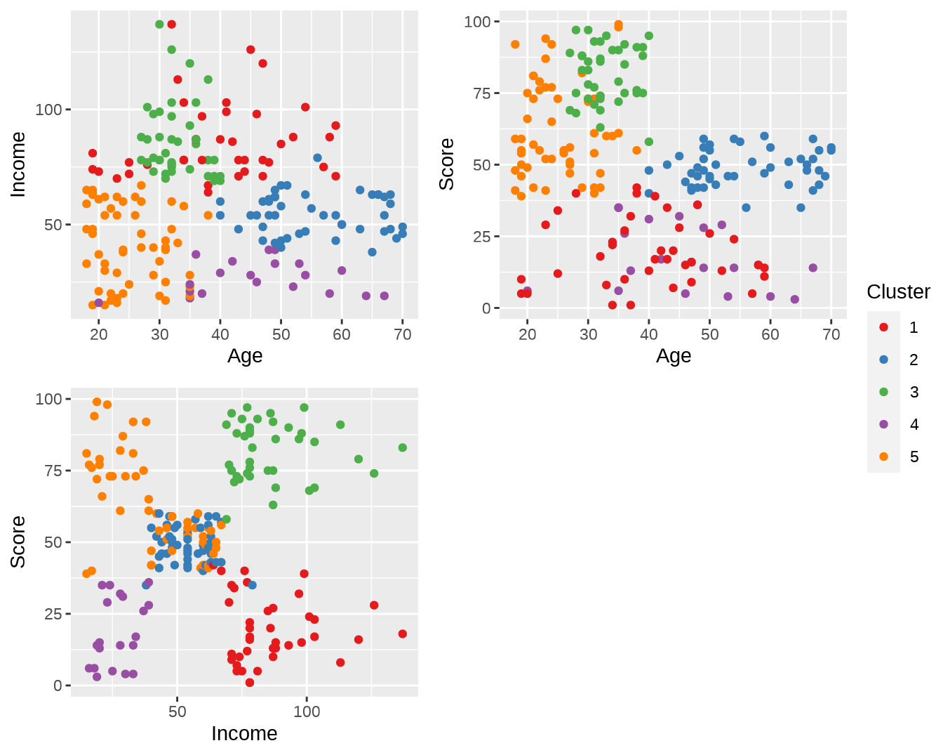
图 6.1: 使用 K-means 聚类后的结果
6.1.2 层次聚类法
接下来使用层次聚类法重做上述任务,并可视化比较两者结果的差别。dist() 默认将计算观测值间的欧氏距离,method = "average" 指定使用平均连接法。plot() 可以直接画出聚类树。
将层级聚类结果切分为 5 个类别。红色的方框叠加显示了各类别的划分。
mall.hclust.cluster = cutree(tree, k = 5)
plot(tree)
rect.hclust(tree, k = 5)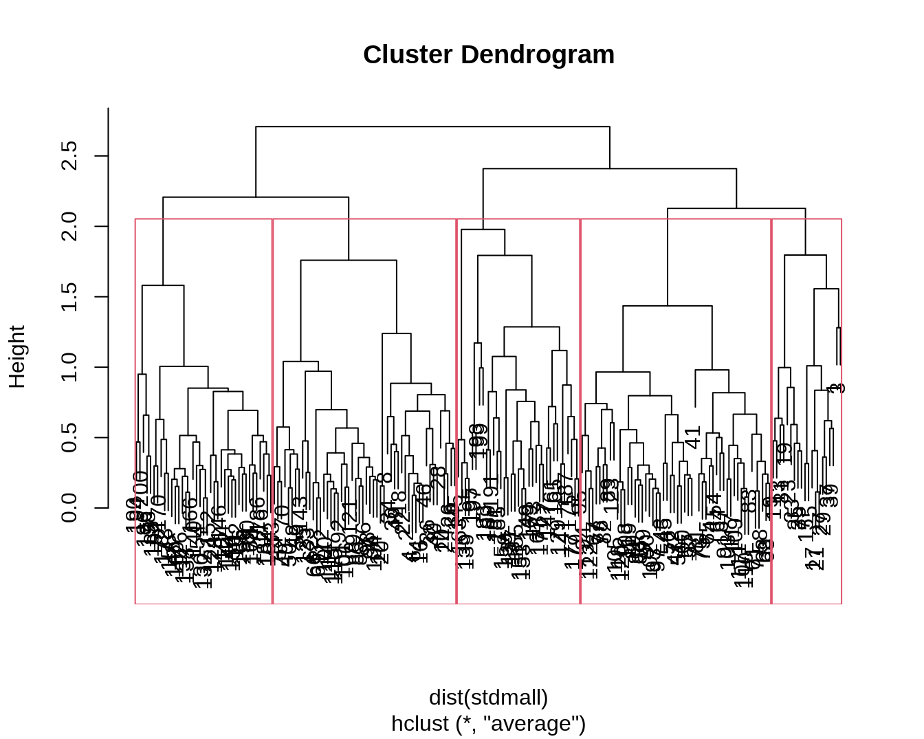
将层次聚类的结果加入原始数据集,并可视化。将两种聚类方法得到的结果放在一起对比,发现基本一致(图 6.2)。
mall.withcluster = mall.withcluster %>%
  mutate(hclust_cluster = as.factor(mall.hclust.cluster))

p = ggplot(mall.withcluster, aes(color = hclust_cluster)) +
  geom_point() +
  scale_color_brewer(palette = "Set1") +
  labs(color = "Cluster")

p4 = p + aes(Age, Income)
p5 = p + aes(Age, Score)
p6 = p + aes(Income, Score)

cowplot::plot_grid(ggpubr::ggarrange(p1, p2, p3, common.legend = TRUE, legend = "right", ncol = 3),
                   ggpubr::ggarrange( p4, p5, p6, common.legend = TRUE, legend = "right", ncol = 3),
                   ncol = 1, labels = "AUTO")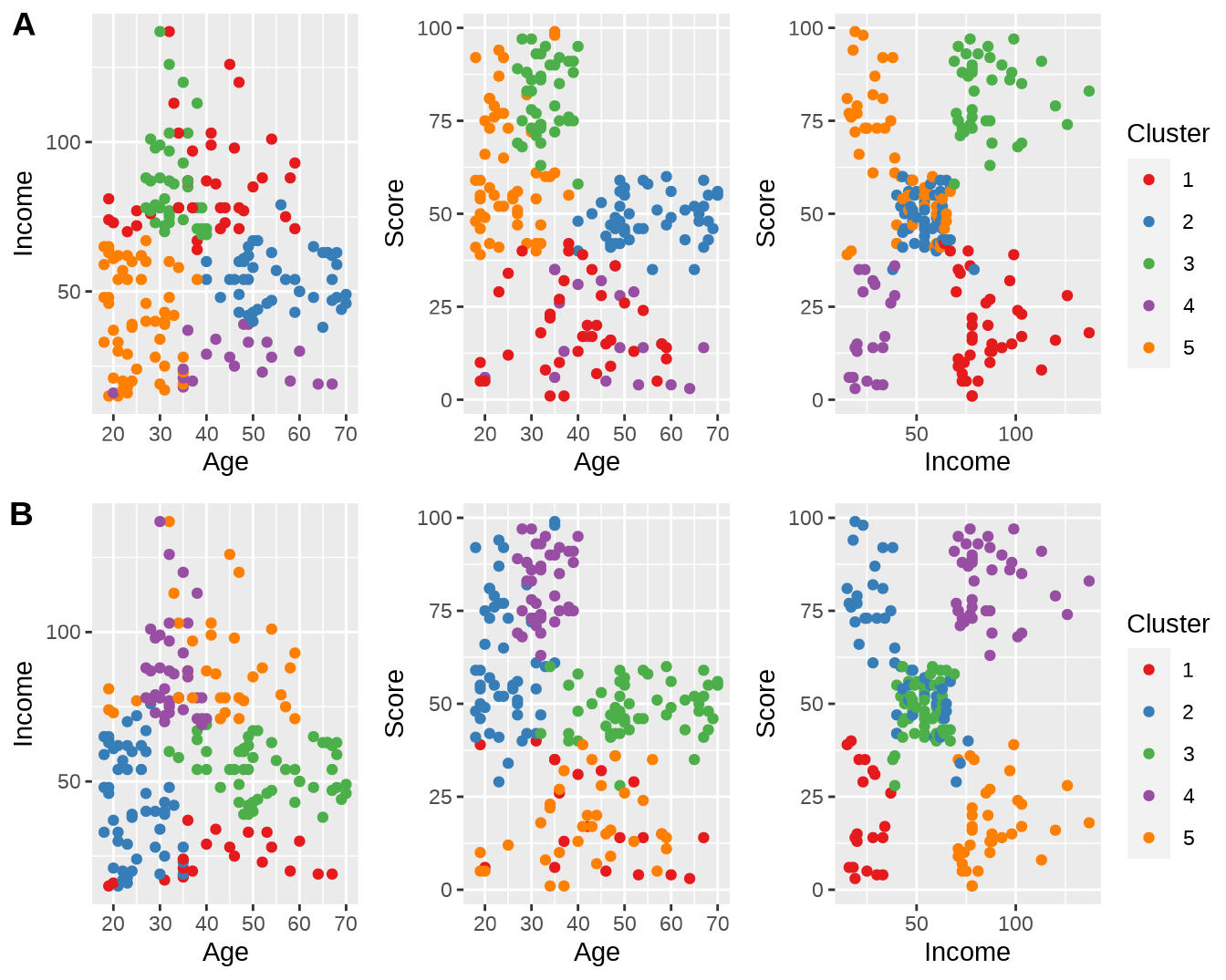
图 6.2: K-means 和 层次聚类结果的比较。
6.1.3 最佳类别数
NbClust 软件包整合了判断最佳类别数的 30 种统计方法,从而能够综合各统计方法的结果得到最佳类别数。
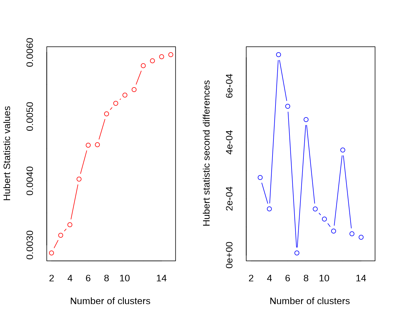
## *** : The Hubert index is a graphical method of determining the number of clusters.
##                 In the plot of Hubert index, we seek a significant knee that corresponds to a
##                 significant increase of the value of the measure i.e the significant peak in Hubert
##                 index second differences plot.
## 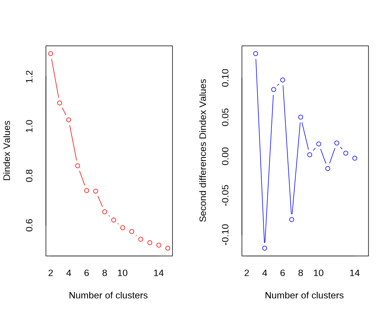
## *** : The D index is a graphical method of determining the number of clusters.
##                 In the plot of D index, we seek a significant knee (the significant peak in Dindex
##                 second differences plot) that corresponds to a significant increase of the value of
##                 the measure.
##
## *******************************************************************
## * Among all indices:
## * 4 proposed 2 as the best number of clusters
## * 3 proposed 3 as the best number of clusters
## * 2 proposed 4 as the best number of clusters
## * 4 proposed 5 as the best number of clusters
## * 4 proposed 6 as the best number of clusters
## * 1 proposed 9 as the best number of clusters
## * 1 proposed 10 as the best number of clusters
## * 2 proposed 12 as the best number of clusters
## * 1 proposed 13 as the best number of clusters
## * 1 proposed 15 as the best number of clusters
##
##                    ***** Conclusion *****
##
## * According to the majority rule, the best number of clusters is  2
##
##
## *******************************************************************
mall.nbclust.kmeans## $All.index
## KL CH Hartigan CCC Scott Marriot TrCovW TraceW
## 2 4.4767 107.0956 63.1628 0.7428 315.5485 5809581 17735.8758 387.4393
## Friedman Rubin Cindex DB Silhouette Duda Pseudot2 Beale Ratkowsky
## 2 2.7054 1.5409 0.3385 1.3557 0.3355 1.1952 -25.6390 -0.2753 0.3427
## Ball Ptbiserial Frey McClain Dunn Hubert SDindex Dindex SDbw
## 2 193.7196 0.4907 0.4209 0.6628 0.0596 0.0029 3.0632 1.2926 1.9128
## [ reached getOption("max.print") -- omitted 13 rows ]
##
## $All.CriticalValues
## CritValue_Duda CritValue_PseudoT2 Fvalue_Beale
## 2 0.5679 119.4765 1.0000
## 3 0.5171 126.0642 1.0000
## 4 0.4304 95.2960 1.0000
## 5 0.4622 77.9553 1.0000
## 6 0.4551 46.7039 0.6456
## 7 0.2298 214.5346 1.0000
## 8 0.4050 60.2358 0.8577
## 9 0.1434 119.4233 1.0000
## 10 0.1148 146.5100 1.0000
## 11 0.4304 48.9716 0.2292
## [ reached getOption("max.print") -- omitted 4 rows ]
##
## $Best.nc
## KL CH Hartigan CCC Scott Marriot TrCovW
## Number_clusters 12.0000 6.0000 4.0000 12.0000 5.0000 5 4.00
## TraceW Friedman Rubin Cindex DB Silhouette Duda
## Number_clusters 3.0000 5.0000 6.0000 9.0000 10.0000 6.0000 2.0000
## PseudoT2 Beale Ratkowsky Ball PtBiserial Frey McClain
## Number_clusters 2.000 2.0000 3.0000 3.0000 5.0000 1 2.0000
## Dunn Hubert SDindex Dindex SDbw
## Number_clusters 15.000 0 6.0000 0 13.0000
## [ reached getOption("max.print") -- omitted 1 row ]
##
## $Best.partition
## [1] 2 2 1 2 2 2 1 2 1 2 1 2 1 2 1 2 1 2 1 2 1 2 1 2 1 2 1 2 1 2
## [ reached getOption("max.print") -- omitted 170 entries ]Best.partition 记录了综合各个统计指标所得的最佳分类结果。
mall.withcluster = mall.withcluster %>%
  mutate(best_kmeans_cluster = as.factor(mall.nbclust.kmeans$Best.partition))
下面使用平均连接层次聚类,并将最佳结果也放到 mall.withcluster 中去。
mall.nbclust.average = NbClust(stdmall, method = "average")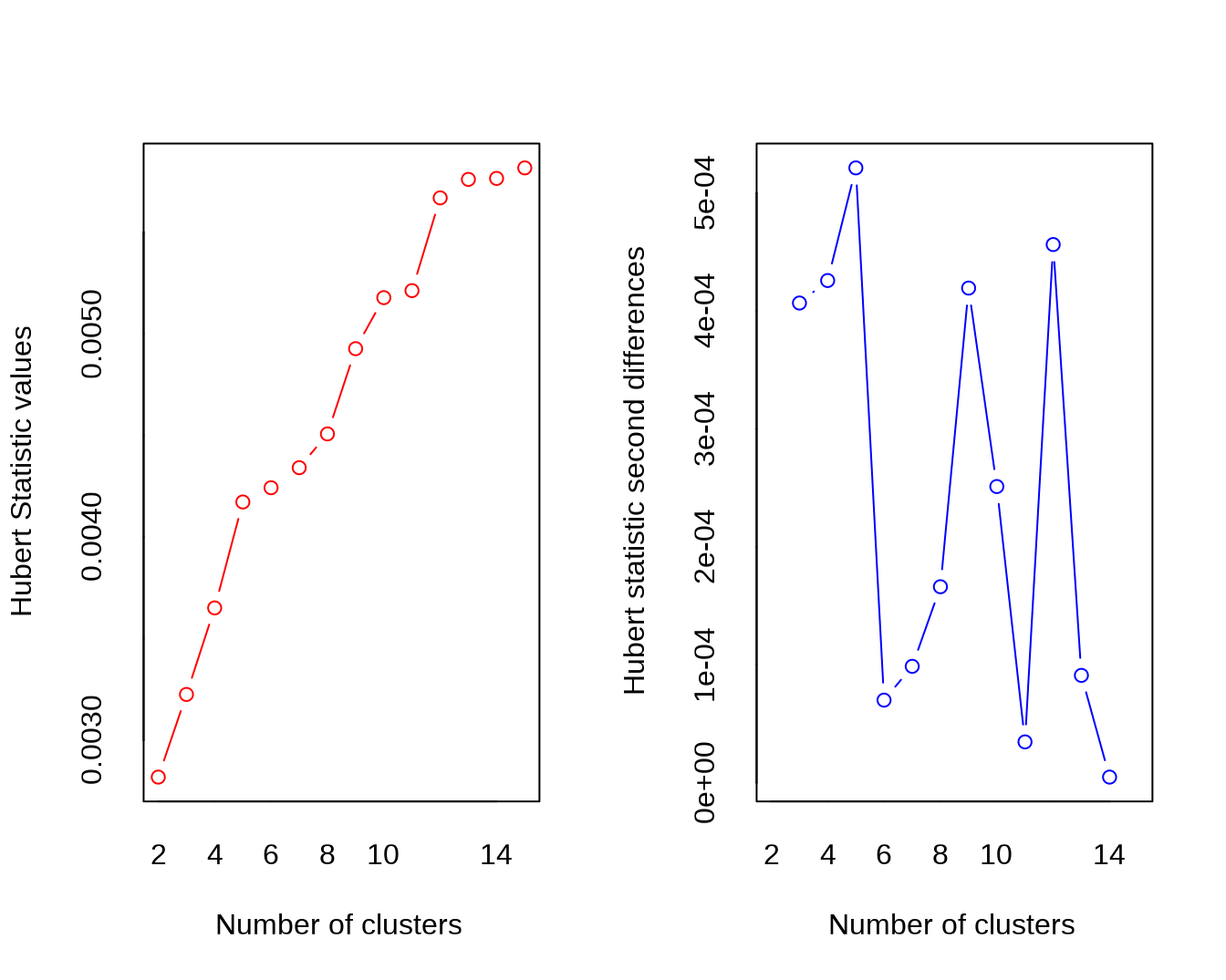
## *** : The Hubert index is a graphical method of determining the number of clusters.
##                 In the plot of Hubert index, we seek a significant knee that corresponds to a
##                 significant increase of the value of the measure i.e the significant peak in Hubert
##                 index second differences plot.
## 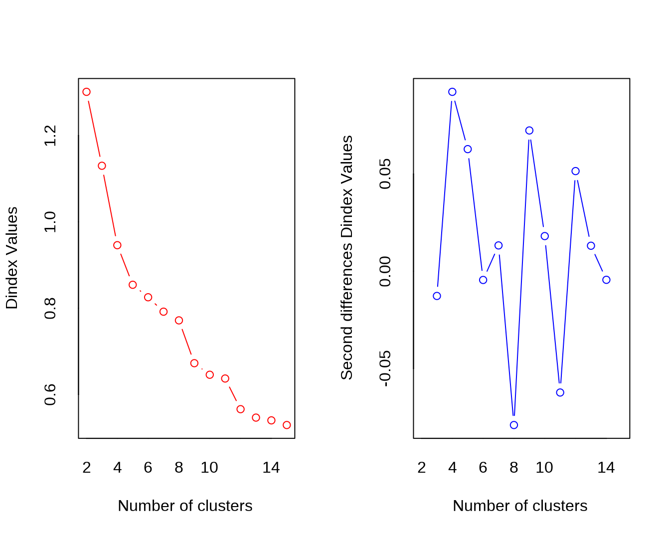
## *** : The D index is a graphical method of determining the number of clusters.
##                 In the plot of D index, we seek a significant knee (the significant peak in Dindex
##                 second differences plot) that corresponds to a significant increase of the value of
##                 the measure.
##
## *******************************************************************
## * Among all indices:
## * 4 proposed 2 as the best number of clusters
## * 3 proposed 3 as the best number of clusters
## * 2 proposed 4 as the best number of clusters
## * 3 proposed 5 as the best number of clusters
## * 1 proposed 6 as the best number of clusters
## * 1 proposed 8 as the best number of clusters
## * 2 proposed 9 as the best number of clusters
## * 1 proposed 11 as the best number of clusters
## * 1 proposed 12 as the best number of clusters
## * 3 proposed 13 as the best number of clusters
## * 2 proposed 15 as the best number of clusters
##
##                    ***** Conclusion *****
##
## * According to the majority rule, the best number of clusters is  2
##
##
## *******************************************************************
mall.withcluster$best_average_cluster = as.factor(mall.nbclust.average$Best.partition)比较最佳类别数下的结果(图 6.3)。
p = ggplot(mall.withcluster) +
  geom_point() +
  scale_color_brewer(palette = "Set1") +
  labs(color = "Cluster")

p7 = p + aes(Age, Income, color = best_kmeans_cluster)
p8 = p + aes(Age, Score, color = best_kmeans_cluster)
p9 = p + aes(Income, Score, color = best_kmeans_cluster)
p10 = p + aes(Age, Income, color = best_average_cluster)
p11 = p + aes(Age, Score, color = best_average_cluster)
p12 = p + aes(Income, Score, color = best_average_cluster)

cowplot::plot_grid(ggpubr::ggarrange(p7, p8, p9, common.legend = TRUE, legend = "right", ncol = 3),
                   ggpubr::ggarrange( p10, p11, p12, common.legend = TRUE, legend = "right", ncol = 3),
                   ncol = 1, labels = "AUTO")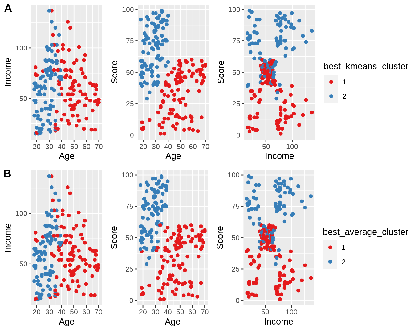
图 6.3: 使用 NbClust 计算得到的最佳类别数聚类后的结果。(A)最佳类别数为 2 的 K-means 聚类;(B)最佳类别数为 2 的层次聚类。