第 5 章 关联规则挖掘
关联规则挖掘常用于购物篮分析应用,目的是发现有意义的强关联规则。
5.1 购物篮分析
使用 arules 软件包自带的 Groceries 交易(transaction)数据集进行购物篮分析。
install.packages("arules")
install.packages("arulesViz")
arules 是用于关联规则挖掘的程序包,我们将调用其中的 itemFrequencyPlot()、apriori()、inspect() 等函数。arulesViz 是用于关联规则可视化的程序包,我们将调用其中的 plot() 函数。
5.1.1 交易数据集的类
Groceries 交易数据集是一个结构化数据,包含了对 169 种商品的 9835 次购买记录。
data("Groceries")
Groceries## transactions in sparse format with
## 9835 transactions (rows) and
## 169 items (columns)
str(Groceries)## Formal class 'transactions' [package "arules"] with 3 slots
## ..@ data :Formal class 'ngCMatrix' [package "Matrix"] with 5 slots
## .. .. ..@ i : int [1:43367] 13 60 69 78 14 29 98 24 15 29 ...
## .. .. ..@ p : int [1:9836] 0 4 7 8 12 16 21 22 27 28 ...
## .. .. ..@ Dim : int [1:2] 169 9835
## .. .. ..@ Dimnames:List of 2
## .. .. .. ..$ : NULL
## .. .. .. ..$ : NULL
## .. .. ..@ factors : list()
## ..@ itemInfo :'data.frame': 169 obs. of 3 variables:
## .. ..$ labels: chr [1:169] "frankfurter" "sausage" "liver loaf" "ham" ...
## .. ..$ level2: Factor w/ 55 levels "baby food","bags",..: 44 44 44 44 44 44 44 42 42 41 ...
## .. ..$ level1: Factor w/ 10 levels "canned food",..: 6 6 6 6 6 6 6 6 6 6 ...
## ..@ itemsetInfo:'data.frame': 0 obs. of 0 variables
summary(Groceries)## transactions as itemMatrix in sparse format with
## 9835 rows (elements/itemsets/transactions) and
## 169 columns (items) and a density of 0.02609146
##
## most frequent items:
## whole milk other vegetables rolls/buns soda
## 2513 1903 1809 1715
## yogurt (Other)
## 1372 34055
##
## element (itemset/transaction) length distribution:
## sizes
## 1 2 3 4 5 6 7 8 9 10 11 12 13 14 15 16
## 2159 1643 1299 1005 855 645 545 438 350 246 182 117 78 77 55 46
## 17 18 19 20 21 22 23 24 26 27 28 29 32
## 29 14 14 9 11 4 6 1 1 1 1 3 1
##
## Min. 1st Qu. Median Mean 3rd Qu. Max.
## 1.000 2.000 3.000 4.409 6.000 32.000
##
## includes extended item information - examples:
## labels level2 level1
## 1 frankfurter sausage meat and sausage
## 2 sausage sausage meat and sausage
## 3 liver loaf sausage meat and sausage使用 head() 和 inspect() 函数可以查看 transactions 对象中的交易数据。
## items
## [1] {citrus fruit,
## semi-finished bread,
## margarine,
## ready soups}
## [2] {tropical fruit,
## yogurt,
## coffee}
## [3] {whole milk}
## [4] {pip fruit,
## yogurt,
## cream cheese ,
## meat spreads}
## [5] {other vegetables,
## whole milk,
## condensed milk,
## long life bakery product}
## [6] {whole milk,
## butter,
## yogurt,
## rice,
## abrasive cleaner}交易数据中,购买次数最多的商品是 whole milk,有超过 2500 次;其次是 other vegetables 等等(图 5.1)。
itemFrequencyPlot(Groceries, topN = 20, type = "absolute")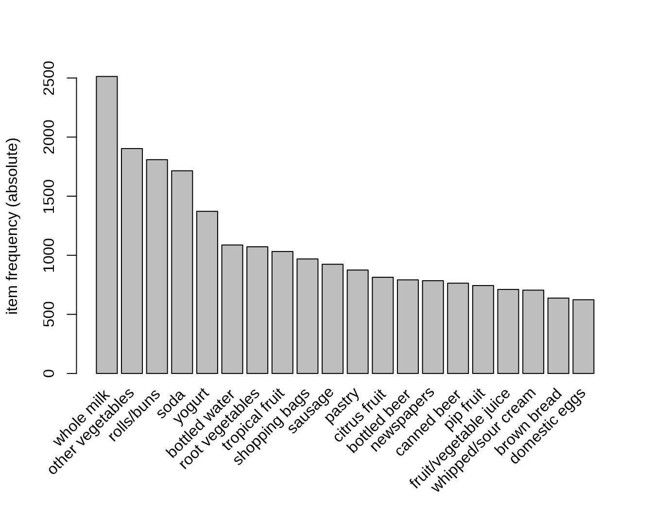
图 5.1: 交易数据集中购买次数最多的 20 项
5.1.2 对交易数据集进行关联分析
apriori() 函数使用 Apriori 算法挖掘关联规则1。函数参数中的 parameter 参数可以指定关联规则的支持度(support),置信度(confidence),每条规则包含的最大项数和最小项数(maxlen/minlen)以及输出结果格式(target)等。
## Apriori
##
## Parameter specification:
## confidence minval smax arem aval originalSupport maxtime support minlen
## 0.8 0.1 1 none FALSE TRUE 5 0.001 1
## maxlen target ext
## 10 rules TRUE
##
## Algorithmic control:
## filter tree heap memopt load sort verbose
## 0.1 TRUE TRUE FALSE TRUE 2 TRUE
##
## Absolute minimum support count: 9
##
## set item appearances ...[0 item(s)] done [0.00s].
## set transactions ...[169 item(s), 9835 transaction(s)] done [0.00s].
## sorting and recoding items ... [157 item(s)] done [0.00s].
## creating transaction tree ... done [0.00s].
## checking subsets of size 1 2 3 4 5 6 done [0.01s].
## writing ... [410 rule(s)] done [0.00s].
## creating S4 object ... done [0.00s].查看输出规则的基本信息,可知:
所生成的关联规则共有 410 条;
关联规则的长度(前项集 lhs 的项数2 + 后项集 rhs 的项数)大多数为 4 或 5;
关联规则的支持度、置信度、提升值和支持观测数的统计值(分位数等)
关联规则挖掘的信息。
summary(rules)## set of 410 rules
##
## rule length distribution (lhs + rhs):sizes
## 3 4 5 6
## 29 229 140 12
##
## Min. 1st Qu. Median Mean 3rd Qu. Max.
## 3.000 4.000 4.000 4.329 5.000 6.000
##
## summary of quality measures:
## support confidence coverage lift
## Min. :0.001017 Min. :0.8000 Min. :0.001017 Min. : 3.131
## 1st Qu.:0.001017 1st Qu.:0.8333 1st Qu.:0.001220 1st Qu.: 3.312
## Median :0.001220 Median :0.8462 Median :0.001322 Median : 3.588
## Mean :0.001247 Mean :0.8663 Mean :0.001449 Mean : 3.951
## 3rd Qu.:0.001322 3rd Qu.:0.9091 3rd Qu.:0.001627 3rd Qu.: 4.341
## Max. :0.003152 Max. :1.0000 Max. :0.003559 Max. :11.235
## count
## Min. :10.00
## 1st Qu.:10.00
## Median :12.00
## Mean :12.27
## 3rd Qu.:13.00
## Max. :31.00
##
## mining info:
## data ntransactions support confidence
## Groceries 9835 0.001 0.8
## call
## apriori(data = Groceries, parameter = list(support = 0.001, confidence = 0.8, target = "rules"))按照提升值(lift)取关联规则的前 3 项,结果显示由项集 \(A\)({liquor, red/blush wine}) 指向项集 \(B\)({bottled beer} )提升值最高。
## lhs rhs support confidence coverage lift count
## [1] {liquor,
## red/blush wine} => {bottled beer} 0.001931876 0.9047619 0.002135231 11.23527 19
## [2] {citrus fruit,
## other vegetables,
## soda,
## fruit/vegetable juice} => {root vegetables} 0.001016777 0.9090909 0.001118454 8.34040 10
## [3] {tropical fruit,
## other vegetables,
## whole milk,
## yogurt,
## oil} => {root vegetables} 0.001016777 0.9090909 0.001118454 8.34040 10图 5.2 对关联规则的可视化结果中可以看出,在全部的 410 个强关联规则中,存在一些支持度(横轴)、置信度(纵轴)和提升值(颜色)均比较理想的规则。
plot(rules)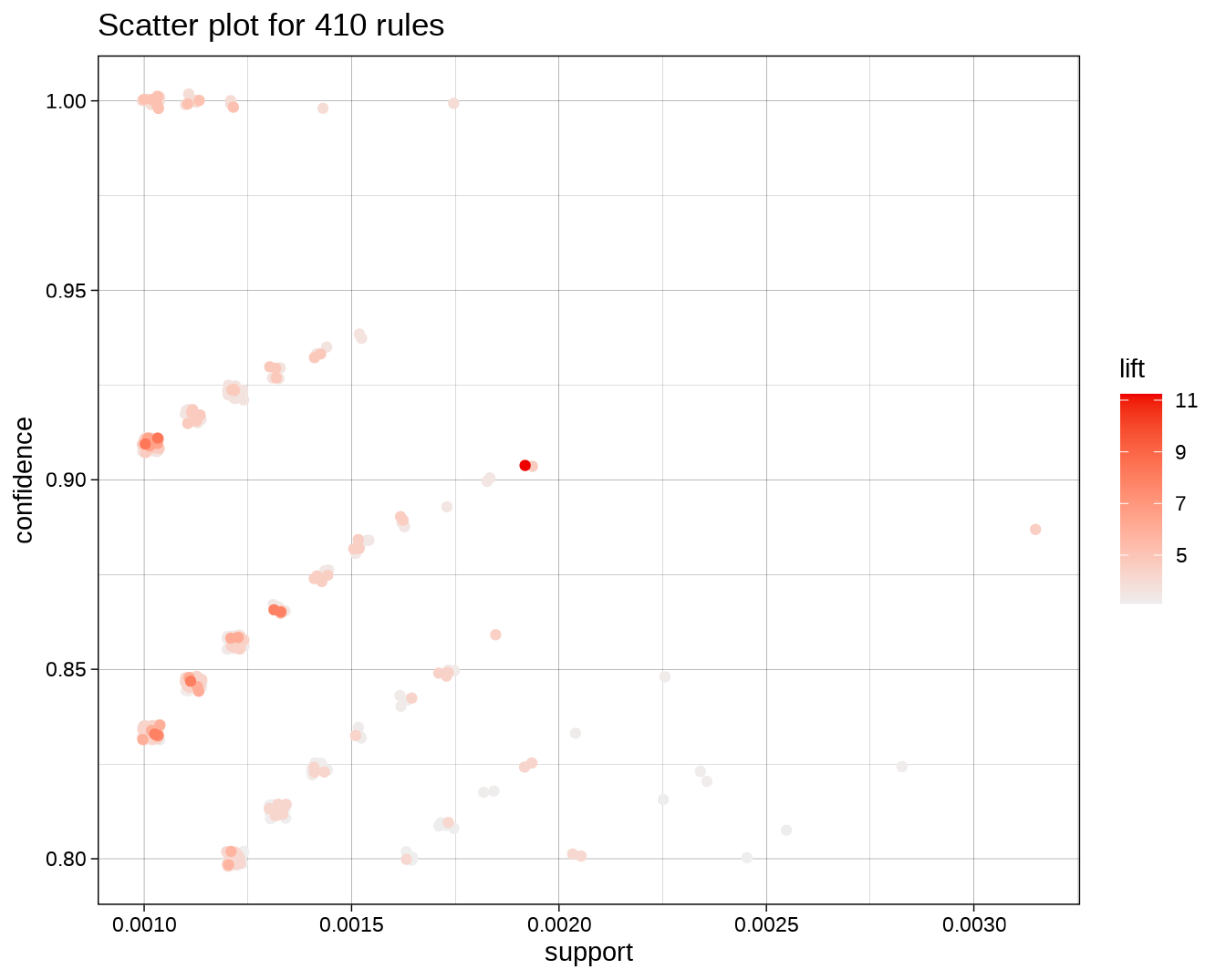
图 5.2: 关联规则的可视化
5.1.3 对关联规则去冗余
关联规则中可能有一些是冗余的。举例来说:假设有一个规则 {A, B, C, D, E} => {F},其置信度为 0.9;另有一条规则 {A, B, C, D} => {F},其置信度为 0.95。因为后面这个规则的一般化程度和置信度都更高,所以前一条就是冗余的规则。除了置信度,还可以用提升值来判断一条规则是否冗余。
# 去冗余
rules_pruned = rules[!is.redundant(rules)]5.1.4 对关联规则进行排序和控制
根据置信度对输出规则进行排序。
rules = sort(rules, by = "confidence", decreasing = TRUE)控制关联规则的长度。
# 指定规则长度最大为 3
rules_maxlen = apriori(
Groceries,
parameter = list(
supp = 0.001,
conf = 0.8,
maxlen = 3
)
)## Apriori
##
## Parameter specification:
## confidence minval smax arem aval originalSupport maxtime support minlen
## 0.8 0.1 1 none FALSE TRUE 5 0.001 1
## maxlen target ext
## 3 rules TRUE
##
## Algorithmic control:
## filter tree heap memopt load sort verbose
## 0.1 TRUE TRUE FALSE TRUE 2 TRUE
##
## Absolute minimum support count: 9
##
## set item appearances ...[0 item(s)] done [0.00s].
## set transactions ...[169 item(s), 9835 transaction(s)] done [0.00s].
## sorting and recoding items ... [157 item(s)] done [0.00s].
## creating transaction tree ... done [0.00s].
## checking subsets of size 1 2 3 done [0.00s].
## writing ... [29 rule(s)] done [0.00s].
## creating S4 object ... done [0.00s].## lhs rhs support confidence
## [1] {liquor, red/blush wine} => {bottled beer} 0.001931876 0.9047619
## [2] {grapes, onions} => {other vegetables} 0.001118454 0.9166667
## coverage lift count
## [1] 0.002135231 11.235269 19
## [2] 0.001220132 4.737476 115.1.5 指定前项集和后项集
指定前项集可以探索顾客在购买了某一商品后,可能会继续购买什么商品。如下面的例子,可以发现用户在购买了 whole milk 后,更有可能去买点蔬菜、酸奶等商品(图 5.3)。
rules_lhs_wholemilk = apriori(
Groceries,
parameter = list(
supp = 0.001,
conf = 0.15
),
appearance = list(
lhs = "whole milk"
),
control = list(
verbose = FALSE
)
)
plot(head(rules_lhs_wholemilk,by = "lift"), method = "graph")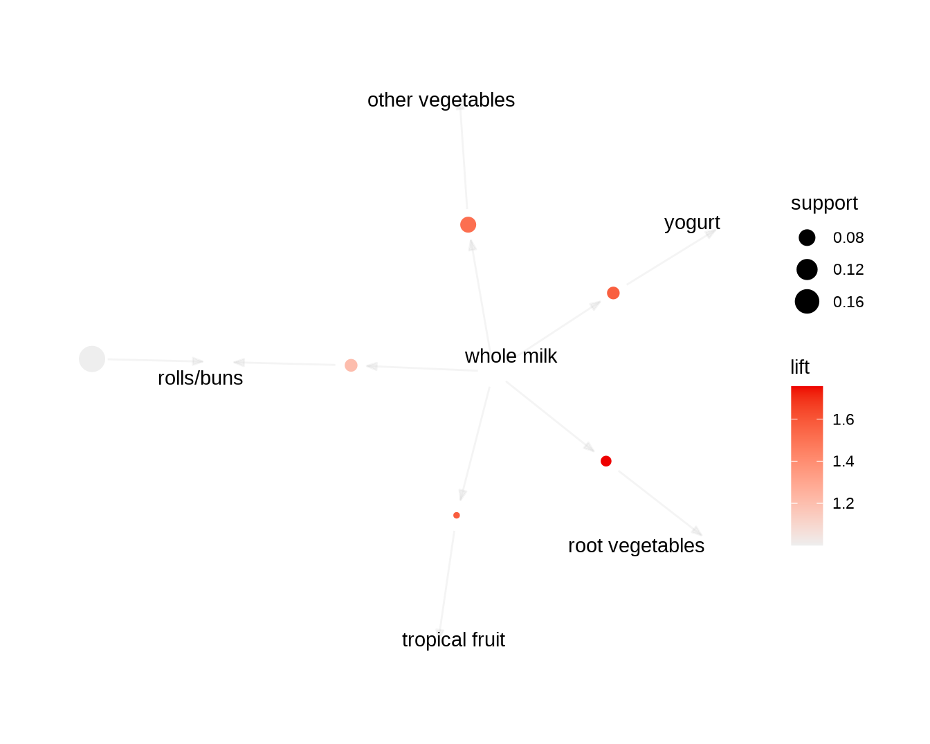
图 5.3: 指定前项集的关联规则
指定后项集可以探索顾客在什么情况下会去买一个商品。如下面的例子,可以发现用户在购买了 点 whipped/sour cream、root vegetables 等商品后,更有可能去买 whole milk(图 5.4)。
rules_rhs_wholemilk = apriori(
Groceries,
parameter = list(
supp = 0.001,
conf = 0.8
),
appearance = list(
rhs = "whole milk"
),
control = list(
verbose = FALSE
)
)
plot(head(rules_rhs_wholemilk,by = "lift"), method = "graph")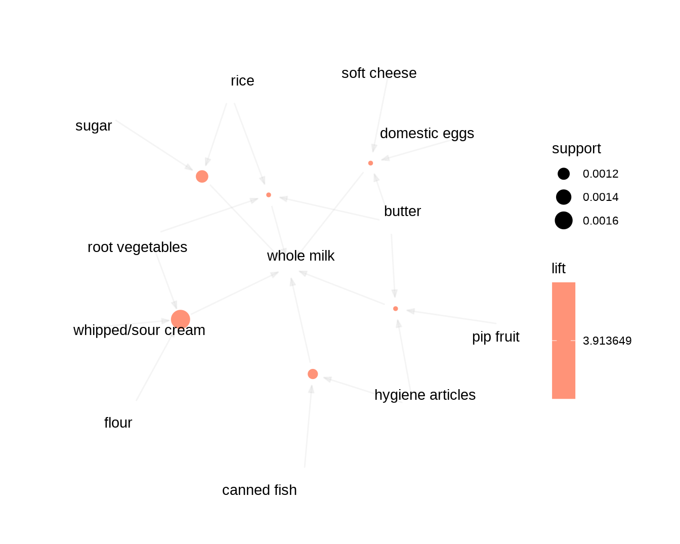
图 5.4: 指定后项集的关联规则
5.2 泰坦尼克号存活情况分析
5.2.1 数据集的定义和预处理
本分析所用的数据集记录了 891 位泰坦尼克号乘客的 12 个变量信息,希望能够通过分析挖掘乘客的存活情况与其它变量的关联规则。
library(readr)
file = xfun::magic_path("ch4_titanic_train.csv")
titanic = read_csv(file)该数据集包含的字段如下:
- PassengerId:乘客编号
- Survived:是否存活(0 = 没有,1 = 存活)
- Pclass:船舱等级(1 = 一等舱,2 = 二等舱,3 = 三等舱)
- Name:乘客姓名
- Sex:乘客性别
- Age:乘客年龄
- Sibsp:船上的兄妹/配偶数目
- Parch:船上的父母/孩子数目
- Ticket:船票号
- Fare:船票价格
- Cabin:船舱号
- Embarked:登船港口(C = 瑟堡,Q = 皇后镇,S = 南安普顿)
summary(titanic)## PassengerId Survived Pclass Name
## Min. : 1.0 Min. :0.0000 Min. :1.000 Length:891
## 1st Qu.:223.5 1st Qu.:0.0000 1st Qu.:2.000 Class :character
## Sex Age SibSp Parch
## Length:891 Min. : 0.42 Min. :0.000 Min. :0.0000
## Class :character 1st Qu.:20.12 1st Qu.:0.000 1st Qu.:0.0000
## Ticket Fare Cabin Embarked
## Length:891 Min. : 0.00 Length:891 Length:891
## Class :character 1st Qu.: 7.91 Class :character Class :character
## [ reached getOption("max.print") -- omitted 5 rows ]在进行关联规则分析前,对数据集进行如下预处理:
- 去掉唯一标识符字段,如乘客编号(PassengerId)、姓名(Name)、传票号(Ticket);
- 去掉缺失过多的字段,如船舱号(Cabin);
- 去掉冗余的字段,如因为船票价格(Fare)与船舱等级相关(Pclass),故删去;
- 删掉一些不完整的记录,如年龄(Age)缺失的观测。
经过这些处理后,还有 712 条观测数据,每个观测有 7 个值。
library(dplyr)
titanic = titanic %>%
select(-c(PassengerId, Name, Ticket, Cabin, Fare)) %>%
mutate_if(is.character, list(~na_if(., ""))) %>% # 将空字符串替换为 NA
filter(complete.cases(.))
titanic## # A tibble: 712 × 7
## Survived Pclass Sex Age SibSp Parch Embarked
## <dbl> <dbl> <chr> <dbl> <dbl> <dbl> <chr>
## 1 0 3 male 22 1 0 S
## 2 1 1 female 38 1 0 C
## 3 1 3 female 26 0 0 S
## 4 1 1 female 35 1 0 S
## 5 0 3 male 35 0 0 S
## 6 0 1 male 54 0 0 S
## 7 0 3 male 2 3 1 S
## 8 1 3 female 27 0 2 S
## 9 1 2 female 14 1 0 C
## 10 1 3 female 4 1 1 S
## # … with 702 more rows
## # ℹ Use `print(n = ...)` to see more rows因为关联分析需要所有的变量均为分类变量(因子),所以需要把年龄(Age)切分为因子。在进行这一操作之前,先看一下年龄的分布情况。
library(ggplot2)
ggplot(titanic, aes(Age)) +
geom_histogram(binwidth = 5, fill = "lightblue", color = "black")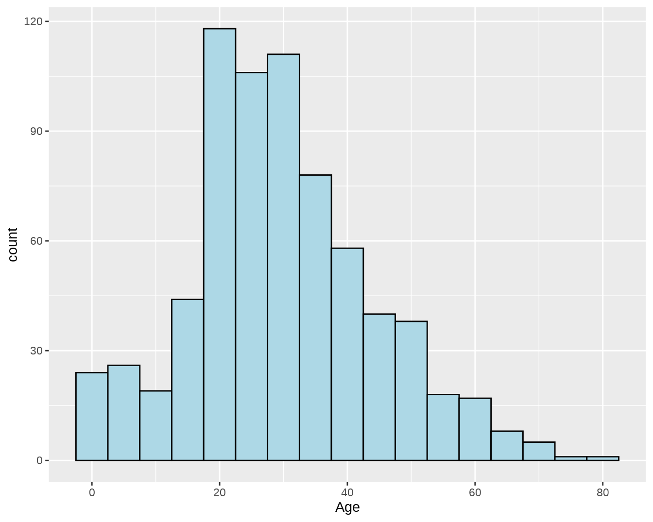
接下来将年龄以 20 岁为间隔切分,并将所有变量转变为因子。
5.2.2 关联规则分析
接下来使用 apriori() 函数对 titanic 数据集进行关联分析。
library(arules)
library(arulesViz)
rules = apriori(titanic, parameter = list(
support = 0.1,
confidence = 0.8
))## Apriori
##
## Parameter specification:
## confidence minval smax arem aval originalSupport maxtime support minlen
## 0.8 0.1 1 none FALSE TRUE 5 0.1 1
## maxlen target ext
## 10 rules TRUE
##
## Algorithmic control:
## filter tree heap memopt load sort verbose
## 0.1 TRUE TRUE FALSE TRUE 2 TRUE
##
## Absolute minimum support count: 71
##
## set item appearances ...[0 item(s)] done [0.00s].
## set transactions ...[27 item(s), 712 transaction(s)] done [0.00s].
## sorting and recoding items ... [16 item(s)] done [0.00s].
## creating transaction tree ... done [0.00s].
## checking subsets of size 1 2 3 4 5 6 7 done [0.00s].
## writing ... [253 rule(s)] done [0.00s].
## creating S4 object ... done [0.00s].
summary(rules)## set of 253 rules
##
## rule length distribution (lhs + rhs):sizes
## 2 3 4 5 6 7
## 8 55 89 67 29 5
##
## Min. 1st Qu. Median Mean 3rd Qu. Max.
## 2.000 4.000 4.000 4.273 5.000 7.000
##
## summary of quality measures:
## support confidence coverage lift
## Min. :0.1011 Min. :0.8030 Min. :0.1110 Min. :1.034
## 1st Qu.:0.1559 1st Qu.:0.8377 1st Qu.:0.1756 1st Qu.:1.115
## Median :0.2191 Median :0.8549 Median :0.2500 Median :1.275
## Mean :0.2326 Mean :0.8706 Mean :0.2692 Mean :1.262
## 3rd Qu.:0.2851 3rd Qu.:0.9027 3rd Qu.:0.3258 3rd Qu.:1.369
## Max. :0.5646 Max. :1.0000 Max. :0.6587 Max. :2.383
## count
## Min. : 72.0
## 1st Qu.:111.0
## Median :156.0
## Mean :165.6
## 3rd Qu.:203.0
## Max. :402.0
##
## mining info:
## data ntransactions support confidence
## titanic 712 0.1 0.8
## call
## apriori(data = titanic, parameter = list(support = 0.1, confidence = 0.8))
plot(rules)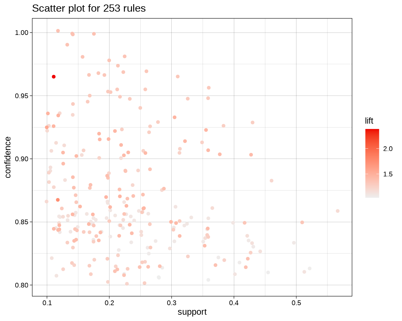
rules = rules[is.redundant(rules)]
inspect(head(rules, by = "lift"))
## lhs rhs support confidence coverage lift count
## [1] {Pclass=3,
## Sex=male,
## SibSp=0,
## Parch=0,
## Embarked=S} => {Survived=0} 0.1952247 0.8687500 0.2247191 1.458844 139
## [2] {Survived=0,
## Pclass=2,
## Embarked=S} => {Sex=male} 0.1067416 0.9268293 0.1151685 1.456738 76
## [3] {Survived=0,
## Age=(20,40],
## SibSp=0,
## Parch=0,
## Embarked=S} => {Sex=male} 0.1797753 0.9208633 0.1952247 1.447361 128
## [4] {Survived=0,
## Age=(20,40],
## SibSp=0,
## Parch=0} => {Sex=male} 0.2106742 0.9202454 0.2289326 1.446390 150
## [5] {Pclass=3,
## Sex=male,
## SibSp=0,
## Parch=0} => {Survived=0} 0.2261236 0.8609626 0.2626404 1.445767 161
## [6] {Pclass=3,
## Sex=male,
## Age=(20,40],
## Parch=0,
## Embarked=S} => {Survived=0} 0.1418539 0.8559322 0.1657303 1.437320 1015.2.3 获救的关联特征
使用指定后项集的关联规则挖掘,可以探究顾客特征取什么值时会存活(Survived = 1)。
rules_rhs_survive = apriori(
  titanic,
  parameter = list(supp = 0.05, conf = 0.8),
  appearance = list(rhs = c("Survived=1")),
  control = list(verbose = FALSE)
)
分析显示,头等舱、女性、无父母和子女的乘客获救的提升值最高,总体有 98.1% 的几率存活;头等舱、女性、年龄 20 - 40 岁的乘客则有 97.7% 的几率存活。
rules_rhs_survive = rules_rhs_survive[!is.redundant(rules_rhs_survive)]
inspect(head(rules_rhs_survive, by = "lift"))
## lhs rhs support confidence
## [1] {Pclass=1, Sex=female, Parch=0} => {Survived=1} 0.07443820 0.9814815
## [2] {Pclass=1, Sex=female, Age=(20,40]} => {Survived=1} 0.06039326 0.9772727
## [3] {Pclass=1, Sex=female, SibSp=0} => {Survived=1} 0.06039326 0.9772727
## coverage lift count
## [1] 0.07584270 2.426440 53
## [2] 0.06179775 2.416035 43
## [3] 0.06179775 2.416035 43
## [ reached 'max' / getOption("max.print") -- omitted 3 rows ]5.2.4 死亡的关联特征
分析乘客死亡的关联特征,可以得出:具有二等舱、男性、年龄在 20 - 40 岁、无兄弟姐妹的乘客死亡几率可达 95%。
rules_rhs_not_survive = apriori(
  titanic,
  parameter = list(supp = 0.05, conf = 0.8),
  appearance = list(rhs = c("Survived=0")),
  control = list(verbose = FALSE)
)
rules_rhs_not_survive = rules_rhs_not_survive[!is.redundant(rules_rhs_not_survive)]
inspect(head(rules_rhs_not_survive, by = "lift"))
## lhs rhs support confidence coverage lift count
## [1] {Pclass=2,
## Sex=male,
## Age=(20,40],
## SibSp=0} => {Survived=0} 0.05337079 0.9500000 0.05617978 1.595283 38
## [2] {Pclass=2,
## Sex=male,
## Age=(20,40]} => {Survived=0} 0.07865169 0.9491525 0.08286517 1.593860 56
## [3] {Pclass=2,
## Sex=male,
## Parch=0} => {Survived=0} 0.10393258 0.9250000 0.11235955 1.553302 74
## [4] {Sex=male,
## Age=(0,20],
## SibSp=0,
## Parch=0,
## Embarked=S} => {Survived=0} 0.05477528 0.9069767 0.06039326 1.523036 39
## [5] {Pclass=2,
## Sex=male,
## SibSp=0,
## Embarked=S} => {Survived=0} 0.08005618 0.9047619 0.08848315 1.519317 57
## [6] {Sex=male,
## Age=(0,20],
## Parch=0,
## Embarked=S} => {Survived=0} 0.06039326 0.8958333 0.06741573 1.504324 435.3 学生特征及考试成绩
StudentsPerformance.csv 数据集给出了一些学生的特征及考试成绩。数据的定义如下:
- gender:性别
- race/ethnicity:种族
- parental level of education:父母教育水平
- lunch:参与的午餐计划
- test preparation course:测验准备课程完成情况
- math score:数学成绩
- reading score:阅读成绩
- writing score:写作成绩
file = xfun::magic_path("StudentsPerformance.csv")
studentPerformance = readr::read_csv(file)
studentPerformance
## # A tibble: 1,000 × 8
## gender `race/ethnicity` parental leve…¹ lunch test …² math …³ readi…⁴ writi…⁵
## <chr> <chr> <chr> <chr> <chr> <dbl> <dbl> <dbl>
## 1 female group B bachelor's deg… stan… none 72 72 74
## 2 female group C some college stan… comple… 69 90 88
## 3 female group B master's degree stan… none 90 95 93
## 4 male group A associate's de… free… none 47 57 44
## 5 male group C some college stan… none 76 78 75
## 6 female group B associate's de… stan… none 71 83 78
## 7 female group B some college stan… comple… 88 95 92
## 8 male group B some college free… none 40 43 39
## 9 male group D high school free… comple… 64 64 67
## 10 female group B high school free… none 38 60 50
## # … with 990 more rows, and abbreviated variable names
## # ¹`parental level of education`, ²`test preparation course`, ³`math score`,
## # ⁴`reading score`, ⁵`writing score`
## # ℹ Use `print(n = ...)` to see more rows将成绩分为不及格(< 60),及格(< 85)和优秀(≥ 85)3 个等级,然后做关联规则分析。例如数学成绩及格的一些关联特征如下。
library(dplyr)
studentPerformance = studentPerformance %>%
  mutate_if(is.numeric, ~ cut(., breaks = c(0, 59, 84, 100), include.lowest = TRUE)) %>%
  mutate_all(as.factor)

# 关联分析
rules_rhs_math = apriori(studentPerformance,
                parameter = list(
                  supp = 0.1,
                  conf = 0.5
                ),
                appearance = list(rhs = "math score=(59,84]")
                )
## Apriori
##
## Parameter specification:
## confidence minval smax arem aval originalSupport maxtime support minlen
## 0.5 0.1 1 none FALSE TRUE 5 0.1 1
## maxlen target ext
## 10 rules TRUE
##
## Algorithmic control:
## filter tree heap memopt load sort verbose
## 0.1 TRUE TRUE FALSE TRUE 2 TRUE
##
## Absolute minimum support count: 100
##
## set item appearances ...[1 item(s)] done [0.00s].
## set transactions ...[26 item(s), 1000 transaction(s)] done [0.00s].
## sorting and recoding items ... [24 item(s)] done [0.00s].
## creating transaction tree ... done [0.00s].
## checking subsets of size 1 2 3 4 5 6 done [0.00s].
## writing ... [78 rule(s)] done [0.00s].
## creating S4 object ... done [0.00s].## lhs rhs support confidence coverage lift count
## [1] {gender=male,
## reading score=(59,84],
## writing score=(59,84]} => {math score=(59,84]} 0.207 0.8553719 0.242 1.527450 207
## [2] {gender=male,
## test preparation course=none,
## reading score=(59,84],
## writing score=(59,84]} => {math score=(59,84]} 0.120 0.8510638 0.141 1.519757 120
## [3] {gender=male,
## lunch=standard,
## reading score=(59,84],
## writing score=(59,84]} => {math score=(59,84]} 0.143 0.8461538 0.169 1.510989 143
## [4] {gender=male,
## test preparation course=none,
## reading score=(59,84]} => {math score=(59,84]} 0.141 0.8294118 0.170 1.481092 141
## [5] {gender=male,
## reading score=(59,84]} => {math score=(59,84]} 0.233 0.8233216 0.283 1.470217 233
## [6] {gender=male,
## lunch=standard,
## test preparation course=none,
## reading score=(59,84]} => {math score=(59,84]} 0.100 0.8196721 0.122 1.463700 100