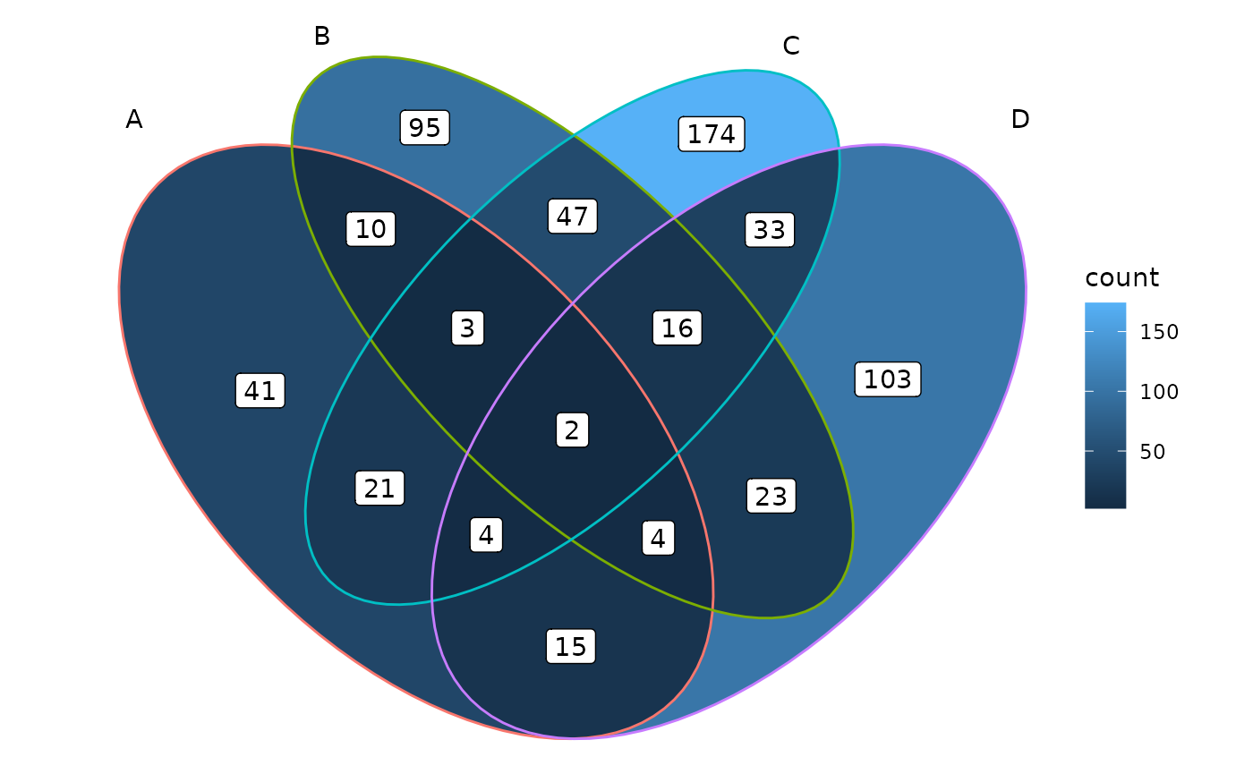
Comprehensive customization by using helper functions
The main function ggVennDiagram() accepts a list input,
and output a ggplot object. By measuring the length of input list, it
automatically applies internal functions to build a plot in two steps:
data preparation and visualization.
Data preparation was packaged into one function
process_data(). Its output is a S4
VennPlotData class object, which contains three slots,
setEdge, setLabel and region.
These slot data then can be further plotted with ggplot
functions.
See below for a better understanding.
Generate example data.
genes <- paste0("gene",1:1000)
set.seed(20231214)
gene_list <- list(A = sample(genes,100),
                  B = sample(genes,200),
                  C = sample(genes,300),
D = sample(genes,200))Then we can reproduce the plot of ggVennDiagram() with
several lines.
venn <- Venn(gene_list)
data <- process_data(venn)
ggplot() +
  # 1. region count layer
  geom_polygon(aes(X, Y, fill = count, group = id),
          data = venn_regionedge(data)) +
  # 2. set edge layer
  geom_path(aes(X, Y, color = id, group = id),
          data = venn_setedge(data),
          show.legend = FALSE) +
  # 3. set label layer
  geom_text(aes(X, Y, label = name),
               data = venn_setlabel(data)) +
  # 4. region label layer
  geom_label(aes(X, Y, label = count),
                data = venn_regionlabel(data)) +
  coord_equal() +
  theme_void()
The variable data is a structured list that has three
slots.
data
#> Class VennPlotData - '401f'
#>   Type: ellipse; No. sets: 4; No. regions: 15.
#>   To view this shape, use `plot_shape_edge(get_shape_by_id('401f'))`.
#>   To view its components, use `venn_setedge()`, `venn_setlabel()`, etc.
ggVennDiagram export functions to get these data, and
they can be used for comprehensive customization in user-side.
-
Venn(): Venn object constructor, use this to construct a Venn object from list. -
process_data(): process data with a Venn object -
venn_regionedge(): get region edge data to plot -
venn_regionlabel(): get region label position to plot -
venn_setedge(): get setedge data to plot -
venn_setlabel(): get setlabel data to plot
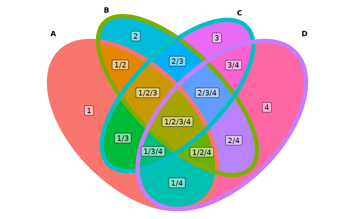
For example, you may change edge/fill/label properties as you will.
ggplot() +
  # change mapping of color filling
  geom_polygon(aes(X, Y, fill = id, group = id),
          data = venn_regionedge(data),
          show.legend = FALSE) +
  # adjust edge size and color
  geom_path(aes(X, Y, color = id, group = id),
          data = venn_setedge(data),
          linewidth = 3,
          show.legend = FALSE) +
  # show set label in bold
  geom_text(aes(X, Y, label = name),
            fontface = "bold",
            data = venn_setlabel(data)) +
  # add a alternative region name
  geom_label(aes(X, Y, label = id),
             data = venn_regionlabel(data),
             alpha = 0.5) +
  coord_equal() +
  theme_void()
Access to classes
set.seed(20231225)
y = list(
  A = sample(letters, 8) |> sort(),
  B = sample(letters, 8) |> sort(),
  C = sample(letters, 8) |> sort(),
  D = sample(letters, 8) |> sort())

# view the list
y
#> $A
#> [1] "a" "e" "g" "o" "p" "s" "t" "v"
#>
#> $B
#> [1] "a" "d" "f" "i" "k" "s" "y" "z"
#>
#> $C
#> [1] "b" "g" "k" "o" "r" "s" "u" "w"
#>
#> $D
#> [1] "b" "c" "e" "h" "k" "q" "s" "y"
Access to subset items
To view subset itmes interactively, set
show_intersect = TRUE.
ggVennDiagram(y, show_intersect = TRUE, set_color = "black")
#> Warning in geom_text(aes(label = .data$count, text = .data$item), data =
#> region_label): Ignoring unknown aesthetics: text
venn_y = Venn(y)

venn_y
#> An object of class 'Venn':
#>    Slots: sets, names;
#>    No. Sets: 4   SetNames: A, B, C, D.
# find the overlaping members of two or more sets
overlap(venn_y, 1:2) # members in both the first two sets
#> [1] "a" "s"
overlap(venn_y) # members in all the sets
#> [1] "s"

# find the different members between sets and set unions
discern(venn_y, 1)  # members in set 1, but not in all the resting sets by default
#> [1] "p" "t" "v"
discern(venn_y, c("A","B"), 3) # members in set A & B, but not in the third set
#>  [1] "a" "e" "p" "t" "v" "d" "f" "i" "y" "z"

# find the specific members in one or more sets
discern_overlap(venn_y, 1)  # specific items in set 1, equals to `discern(venn_y, 1)`. Those members are not shared by all the other sets.
#> [1] "p" "t" "v"
discern_overlap(venn_y, 1:2)  # specific items in set 1 and set 2
#> [1] "a"
Access to plot data
venn_plot_data = process_data(venn_y)

# summary of VennPlotData object
venn_plot_data
#> Class VennPlotData - '401f'
#>   Type: ellipse; No. sets: 4; No. regions: 15.
#>   To view this shape, use `plot_shape_edge(get_shape_by_id('401f'))`.
#>   To view its components, use `venn_setedge()`, `venn_setlabel()`, etc.
Sets and labels
# get the set data
venn_set(venn_plot_data)
#> # A tibble: 4 × 4
#>   id    name  item         count
#>   <chr> <chr> <named list> <int>
#> 1 1     A     <chr [8]>        8
#> 2 2     B     <chr [8]>        8
#> 3 3     C     <chr [8]>        8
#> 4 4     D     <chr [8]>        8

# get subsets, i.e., regions
venn_region(venn_plot_data)
#> # A tibble: 15 × 4
#>    id      name    item      count
#>    <chr>   <chr>   <list>    <int>
#>  1 1       A       <chr [3]>     3
#>  2 2       B       <chr [4]>     4
#>  3 3       C       <chr [3]>     3
#>  4 4       D       <chr [3]>     3
#>  5 1/2     A/B     <chr [1]>     1
#>  6 1/3     A/C     <chr [2]>     2
#>  7 1/4     A/D     <chr [1]>     1
#>  8 2/3     B/C     <chr [0]>     0
#>  9 2/4     B/D     <chr [1]>     1
#> 10 3/4     C/D     <chr [1]>     1
#> 11 1/2/3   A/B/C   <chr [0]>     0
#> 12 1/2/4   A/B/D   <chr [0]>     0
#> 13 1/3/4   A/C/D   <chr [0]>     0
#> 14 2/3/4   B/C/D   <chr [1]>     1
#> 15 1/2/3/4 A/B/C/D <chr [1]>     1
Polygons.
# get set edge
venn_setedge(venn_plot_data)
#> # A tibble: 404 × 3
#>    id         X     Y
#>    <chr>  <dbl> <dbl>
#>  1 1     0.103  0.717
#>  2 1     0.0941 0.708
#>  3 1     0.0867 0.698
#>  4 1     0.0804 0.687
#>  5 1     0.0751 0.675
#>  6 1     0.0709 0.662
#>  7 1     0.0678 0.648
#>  8 1     0.0659 0.634
#>  9 1     0.0650 0.619
#> 10 1     0.0653 0.603
#> # ℹ 394 more rows

# get region edge
venn_regionedge(venn_plot_data)
#> # A tibble: 713 × 6
#>    id        X     Y name  item      count
#>    <chr> <dbl> <dbl> <chr> <list>    <int>
#>  1 1     0.103 0.717 A     <chr [3]>     3
#>  2 1     0.112 0.726 A     <chr [3]>     3
#>  3 1     0.122 0.733 A     <chr [3]>     3
#>  4 1     0.133 0.740 A     <chr [3]>     3
#>  5 1     0.145 0.745 A     <chr [3]>     3
#>  6 1     0.158 0.749 A     <chr [3]>     3
#>  7 1     0.172 0.752 A     <chr [3]>     3
#>  8 1     0.186 0.754 A     <chr [3]>     3
#>  9 1     0.201 0.755 A     <chr [3]>     3
#> 10 1     0.217 0.755 A     <chr [3]>     3
#> # ℹ 703 more rows
df = venn_setedge(venn_plot_data)
plot(df$X, df$Y, asp = 1)